The Scientist and Engineer's Guide to
Digital Signal Processing
By Steven W. Smith, Ph.D.
Book Search

Table of contents
- 1: The Breadth and Depth of DSP
- 2: Statistics, Probability and Noise
- 3: ADC and DAC
- 4: DSP Software
- 5: Linear Systems
- 6: Convolution
- 7: Properties of Convolution
- 8: The Discrete Fourier Transform
- 9: Applications of the DFT
- 10: Fourier Transform Properties
- 11: Fourier Transform Pairs
- 12: The Fast Fourier Transform
- 13: Continuous Signal Processing
- 14: Introduction to Digital Filters
- 15: Moving Average Filters
- 16: Windowed-Sinc Filters
- 17: Custom Filters
- 18: FFT Convolution
- 19: Recursive Filters
- 20: Chebyshev Filters
- 21: Filter Comparison
- 22: Audio Processing
- 23: Image Formation & Display
- 24: Linear Image Processing
- 25: Special Imaging Techniques
- 26: Neural Networks (and more!)
- 27: Data Compression
- 28: Digital Signal Processors
- 29: Getting Started with DSPs
- 30: Complex Numbers
- 31: The Complex Fourier Transform
- 32: The Laplace Transform
- 33: The z-Transform
- 34: Explaining Benford's Law
How to order your own hardcover copy
Wouldn't you rather have a bound book instead of 640 loose pages?Your laser printer will thank you!
Order from Amazon.com.
Chapter 27: Data Compression
Many methods of lossy compression have been developed; however, a family of techniques called transform compression has proven the most valuable. The best example of transform compression is embodied in the popular JPEG standard of image encoding. JPEG is named after its origin, the Joint Photographers Experts Group. We will describe the operation of JPEG to illustrate how lossy compression works.
We have already discussed a simple method of lossy data compression, coarser sampling and/or quantization (CS&Q in Table 27-1). This involves reducing the number of bits per sample or entirely discard some of the samples. Both these procedures have the desired effect: the data file becomes smaller at the expense of signal quality. As you might expect, these simple methods do not work very well.
Transform compression is based on a simple premise: when the signal is passed through the Fourier (or other) transform, the resulting data values will no longer be equal in their information carrying roles. In particular, the low frequency components of a signal are more important than the high frequency components. Removing 50% of the bits from the high frequency components might remove, say, only 5% of the encoded information.
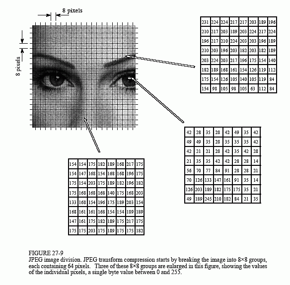
As shown in Fig. 27-9, JPEG compression starts by breaking the image into 8×8 pixel groups. The full JPEG algorithm can accept a wide range of bits per pixel, including the use of color information. In this example, each pixel is a single byte, a grayscale value between 0 and 255. These 8×8 pixel groups are treated independently during compression. That is, each group is initially represented by 64 bytes. After transforming and removing data, each group is represented by, say, 2 to 20 bytes. During uncompression, the inverse transform is taken of the 2 to 20 bytes to create an approximation of the original 8×8 group. These approximated groups are then fitted together to form the uncompressed image. Why use 8×8 pixel groups instead of, for instance, 16×16? The 8×8 grouping was based on the maximum size that integrated circuit technology could handle at the time the standard was developed. In any event, the 8×8 size works well, and it may or may not be changed in the future.
Many different transforms have been investigated for data compression, some of them invented specifically for this purpose. For instance, the Karhunen-Loeve transform provides the best possible compression ratio, but is difficult to implement. The Fourier transform is easy to use, but does not provide adequate compression. After much competition, the winner is a relative of the Fourier transform, the Discrete Cosine Transform (DCT).
Just as the Fourier transform uses sine and cosine waves to represent a signal, the DCT only uses cosine waves. There are several versions of the DCT, with slight differences in their mathematics. As an example of one version, imagine a 129 point signal, running from sample 0 to sample 128. Now, make this a 256 point signal by duplicating samples 1 through 127 and adding them as samples 255 to 130. That is: 0, 1, 2, …, 127, 128, 127, …, 2, 1. Taking the Fourier transform of this 256 point signal results in a frequency spectrum of 129 points, spread between 0 and 128. Since the time domain signal was forced to be symmetrical, the spectrum's imaginary part will be composed of all zeros. In other words, we started with a 129 point time domain signal, and ended with a frequency spectrum of 129 points, each the amplitude of a cosine wave. Voila, the DCT!
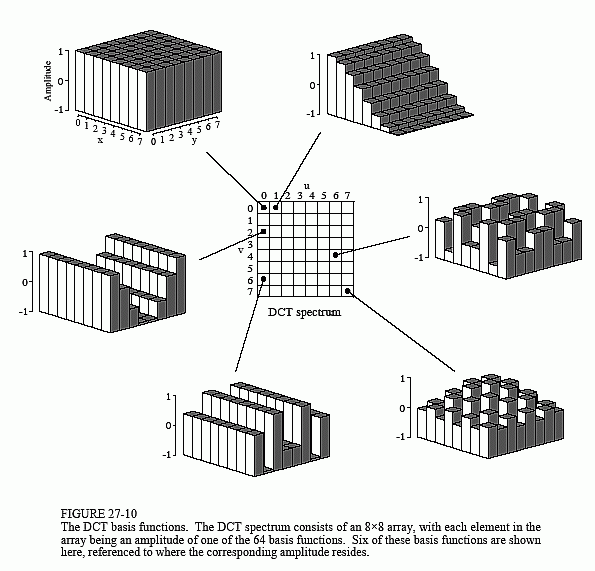
When the DCT is taken of an 8×8 group, it results in an 8×8 spectrum. In other words, 64 numbers are changed into 64 other numbers. All these values are real; there is no complex mathematics here. Just as in Fourier analysis, each value in the spectrum is the amplitude of a basis function. Figure 27-10 shows 6 of the 64 basis functions used in an 8×8 DCT, according to where the amplitude sits in the spectrum. The 8×8 DCT basis functions are given by:

The low frequencies reside in the upper-left corner of the spectrum, while the high frequencies are in the lower-right. The DC component is at [0,0], the upper-left most value. The basis function for [0,1] is one-half cycle of a cosine wave in one direction, and a constant value in the other. The basis function for [1,0] is similar, just rotated by 90°.
The DCT calculates the spectrum by correlating the 8×8 pixel group with each of the basis functions. That is, each spectral value is found by multiplying the appropriate basis function by the 8×8 pixel group, and then summing the products. Two adjustments are then needed to finish the DCT calculation (just as with the Fourier transform). First, divide the 15 spectral values in row 0 and column 0 by two. Second, divide all 64 values in the spectrum by 16. The inverse DCT is calculated by assigning each of the amplitudes in the spectrum to the proper basis function, and summing to recreate the spatial domain. No extra steps are required. These are exactly the same concepts as in Fourier analysis, just with different basis functions.
Figure 27-11 illustrates JPEG encoding for the three 8×8 groups identified
in Fig. 27-9. The left column, Figs. a, b & c, show the original pixel values. The center column, Figs. d, e & f, show the DCT spectra of these groups.
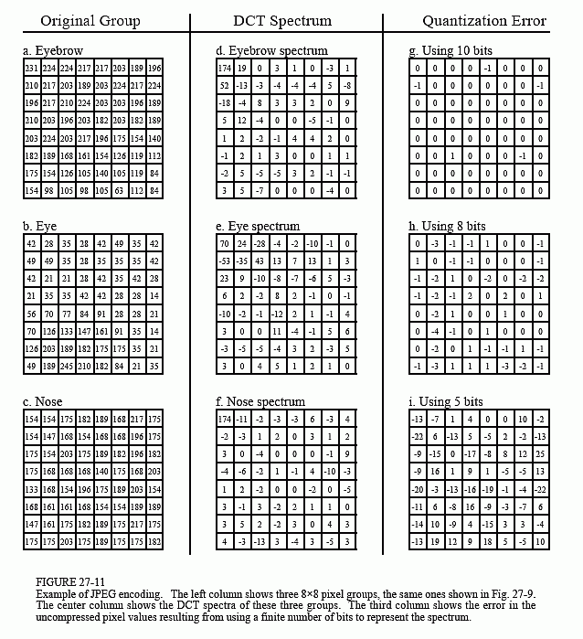
The right column, Figs. g, h & i, shows the effect of reducing the number of bits used to represent each component in the frequency spectrum. For instance, (g) is formed by truncating each of the samples in (d) to ten bits, taking the inverse DCT, and then subtracting the reconstructed image from the original. Likewise, (h) and (i) are formed by truncating each sample in the spectrum to eight and five bits, respectively. As expected, the error in the reconstruction increases as fewer bits are used to represent the data. As an example of this bit truncation, the spectra shown in the center column are represented with 8 bits per spectral value, arranged as 0 to 255 for the DC component, and -127 to 127 for the other values.
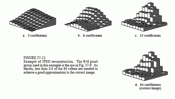
The second method of compressing the frequency domain is to discard some of the 64 spectral values. As shown by the spectra in Fig. 27-11, nearly all of the signal is contained in the low frequency components. This means the highest frequency components can be eliminated, while only degrading the signal a small amount. Figure 27-12 shows an example of the image distortion that occurs when various numbers of the high frequency components are deleted. The 8×8 group used in this example is the eye image of Fig. 27-10. Figure (d) shows the correct reconstruction using all 64 spectral values. The remaining figures show the reconstruction using the indicated number of lowest frequency coefficients. As illustrated in (c), even removing three-fourths of the highest frequency components produces little error in the reconstruction. Even better, the error that does occur looks very much like random noise.
JPEG is good example of how several data compression schemes can be combined for greater effectiveness. The entire JPEG procedure is outlined in the following steps. First, the image is broken into the 8×8 groups. Second, the DCT is taken of each group. Third, each 8×8 spectrum is compressed by the above methods: reducing the number of bits and eliminating some of the components. This takes place in a single step, controlled by a quantization table. Two examples of quantization tables are shown in Fig. 27-13. Each value in the spectrum is divided by the matching value in the quantization table, and the result rounded to the nearest integer. For instance, the upper-left value of the quantization table is one,
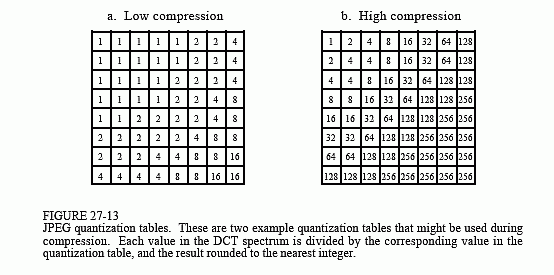
resulting in the DC value being left unchanged. In comparison, the lower-right entry in (a) is 16, meaning that the original range of -127 to 127 is reduced to only -7 to 7. In other words, the value has been reduced in precision from eight bits to four bits. In a more extreme case, the lower-right entry in (b) is 256, completely eliminating the spectral value.
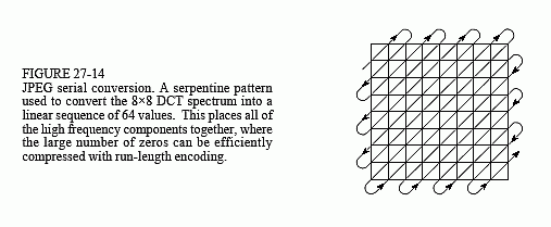
In the fourth step of JPEG encoding, the modified spectrum is converted from an 8×8 array into a linear sequence. The serpentine pattern shown in Figure 27-14 is used for this step, placing all of the high frequency components together at the end of the linear sequence. This groups the zeros from the eliminated components into long runs. The fifth step compresses these runs of zeros by run-length encoding. In the sixth step, the sequence is encoded by either Huffman or arithmetic encoding to form the final compressed file.
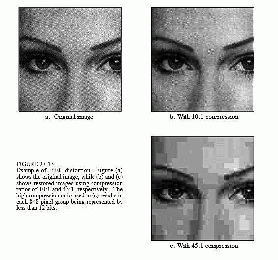
The amount of compression, and the resulting loss of image quality, can be selected when the JPEG compression program is run. Figure 27-15 shows the type of image distortion resulting from high compression ratios. With the 45:1 compression ratio shown, each of the 8×8 groups is represented by only about 12 bits. Close inspection of this image shows that six of the lowest frequency basis functions are represented to some degree.
Why is the DCT better than the Fourier transform for image compression? The main reason is that the DCT has one-half cycle basis functions, i.e., S[0,1] and S[1,0]. As shown in Fig. 27-10, these gently slope from one side of the array to the other. In comparison, the lowest frequencies in the Fourier transform form one complete cycle. Images nearly always contain regions where the brightness is gradually changing over a region. Using a basis function that matches this basic pattern allows for better compression.