The Scientist and Engineer's Guide to
Digital Signal Processing
By Steven W. Smith, Ph.D.
Book Search
Table of contents
- 1: The Breadth and Depth of DSP
- 2: Statistics, Probability and Noise
- 3: ADC and DAC
- 4: DSP Software
- 5: Linear Systems
- 6: Convolution
- 7: Properties of Convolution
- 8: The Discrete Fourier Transform
- 9: Applications of the DFT
- 10: Fourier Transform Properties
- 11: Fourier Transform Pairs
- 12: The Fast Fourier Transform
- 13: Continuous Signal Processing
- 14: Introduction to Digital Filters
- 15: Moving Average Filters
- 16: Windowed-Sinc Filters
- 17: Custom Filters
- 18: FFT Convolution
- 19: Recursive Filters
- 20: Chebyshev Filters
- 21: Filter Comparison
- 22: Audio Processing
- 23: Image Formation & Display
- 24: Linear Image Processing
- 25: Special Imaging Techniques
- 26: Neural Networks (and more!)
- 27: Data Compression
- 28: Digital Signal Processors
- 29: Getting Started with DSPs
- 30: Complex Numbers
- 31: The Complex Fourier Transform
- 32: The Laplace Transform
- 33: The z-Transform
- 34: Explaining Benford's Law
How to order your own hardcover copy
Wouldn't you rather have a bound book instead of 640 loose pages?Your laser printer will thank you!
Order from Amazon.com.
Chapter 25: Special Imaging Techniques
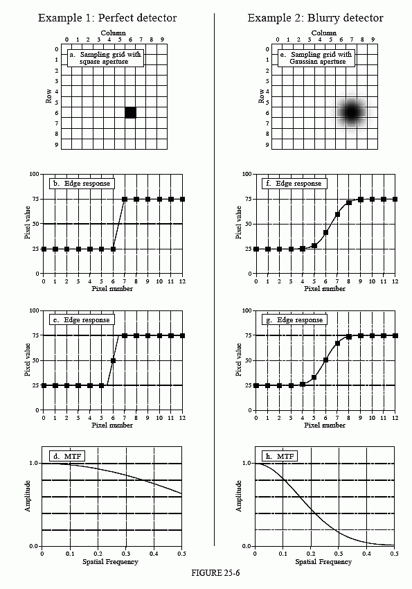
Figure 25-6 shows two extreme examples of sampling, which we will call a perfect detector and a blurry detector. Imagine (a) being the surface of an imaging detector, such as a CCD. Light striking anywhere inside one of the square pixels will contribute only to that pixel value, and no others. This is shown in the figure by the black sampling aperture exactly filling one of the square pixels. This is an optimal situation for an image detector, because all of the light is detected, and there is no overlap or crosstalk between adjacent pixels. In other words, the sampling aperture is exactly equal to the sample spacing.
The alternative example is portrayed in (e). The sampling aperture is considerably larger than the sample spacing, and it follows a Gaussian distribution. In other words, each pixel in the detector receives a contribution from light striking the detector in a region around the pixel. This should sound familiar, because it is the output side viewpoint of convolution. From the corresponding input side viewpoint, a narrow beam of light striking the detector would contribute to the value of several neighboring pixels, also according to the Gaussian distribution.
Now turn your attention to the edge responses of the two examples. The markers in each graph indicate the actual pixel values you would find in an image, while the connecting lines show the underlying curve that is being sampled. An important concept is that the shape of this underlying curve is determined only by the sampling aperture. This means that the resolution in the final image can be limited in two ways. First, the underlying curve may have poor resolution, resulting from the sampling aperture being too large. Second, the sample spacing may be too large, resulting in small details being lost between the samples. Two edge response curves are presented for each example, illustrating that the actual samples can fall anywhere along the underlying curve. In other words, the edge being imaged may be sitting exactly upon a pixel, or be straddling two pixels. Notice that the perfect detector has zero or one sample on the rising part of the edge. Likewise, the blurry detector has three to four samples on the rising part of the edge.
What is limiting the resolution in these two systems? The answer is provided by the sampling theorem. As discussed in Chapter 3, sampling captures all frequency components below one-half of the sampling rate, while higher frequencies are lost due to aliasing. Now look at the MTF curve in (h). The sampling aperture of the blurry detector has removed all frequencies greater than one-half the sampling rate; therefore, nothing is lost during sampling. This means that the resolution of this system is

completely limited by the sampling aperture, and not the sample spacing. Put another way, the sampling aperture has acted as an antialias filter, allowing lossless sampling to take place.
In comparison, the MTF curve in (d) shows that both processes are limiting the resolution of this system. The high-frequency fall-off of the MTF curve represents information lost due to the sampling aperture. Since the MTF curve has not dropped to zero before a frequency of 0.5, there is also information lost during sampling, a result of the finite sample spacing. Which is limiting the resolution more? It is difficult to answer this question with a number, since they degrade the image in different ways. Suffice it to say that the resolution in the perfect detector (example 1) is mostly limited by the sample spacing.
While these concepts may seem difficult, they reduce to a very simple rule for practical usage. Consider a system with some 10%-90% edge response distance, for example 1 mm. If the sample spacing is greater than 1 mm (there is less than one sample along the edge), the system will be limited by the sample spacing. If the sample spacing is less than 0.33 mm (there are more than 3 samples along the edge), the resolution will be limited by the sampling aperture. When a system has 1-3 samples per edge, it will be limited by both factors.
