The Scientist and Engineer's Guide to
Digital Signal Processing
By Steven W. Smith, Ph.D.
Book Search

Table of contents
- 1: The Breadth and Depth of DSP
- 2: Statistics, Probability and Noise
- 3: ADC and DAC
- 4: DSP Software
- 5: Linear Systems
- 6: Convolution
- 7: Properties of Convolution
- 8: The Discrete Fourier Transform
- 9: Applications of the DFT
- 10: Fourier Transform Properties
- 11: Fourier Transform Pairs
- 12: The Fast Fourier Transform
- 13: Continuous Signal Processing
- 14: Introduction to Digital Filters
- 15: Moving Average Filters
- 16: Windowed-Sinc Filters
- 17: Custom Filters
- 18: FFT Convolution
- 19: Recursive Filters
- 20: Chebyshev Filters
- 21: Filter Comparison
- 22: Audio Processing
- 23: Image Formation & Display
- 24: Linear Image Processing
- 25: Special Imaging Techniques
- 26: Neural Networks (and more!)
- 27: Data Compression
- 28: Digital Signal Processors
- 29: Getting Started with DSPs
- 30: Complex Numbers
- 31: The Complex Fourier Transform
- 32: The Laplace Transform
- 33: The z-Transform
- 34: Explaining Benford's Law
How to order your own hardcover copy
Wouldn't you rather have a bound book instead of 640 loose pages?Your laser printer will thank you!
Order from Amazon.com.
Chapter 15: Moving Average Filters
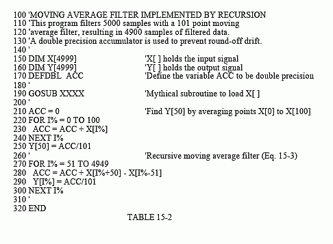
A tremendous advantage of the moving average filter is that it can be implemented with an algorithm that is very fast. To understand this
algorithm, imagine passing an input signal, x[ ], through a seven point moving average filter to form an output signal, y[ ]. Now look at how two adjacent output points, y[50] and y[51], are calculated:
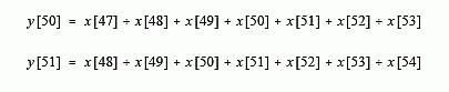
These are nearly the same calculation; points x[48] through x[53] must be added for y[50], and again for y[51]. If y[50] has already been calculated, the most efficient way to calculate y[51] is:
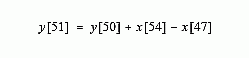
Once y[51] has been found using y[50], then y[52] can be calculated from sample y[51], and so on. After the first point is calculated in y[ ], all of the other points can be found with only a single addition and subtraction per point. This can be expressed in the equation:
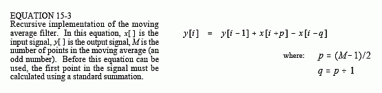
Notice that this equation use two sources of data to calculate each point in the output: points from the input and previously calculated points from the output. This is called a recursive equation, meaning that the result of one calculation is used in future calculations. (The term "recursive" also has other meanings, especially in computer science). Chapter 19 discusses a variety of recursive filters in more detail. Be aware that the moving average recursive filter is very different from typical recursive filters. In particular, most recursive filters have an infinitely long impulse response (IIR), composed of sinusoids and exponentials. The impulse response of the moving average is a rectangular pulse (finite impulse response, or FIR).
This algorithm is faster than other digital filters for several reasons. First, there are only two computations per point, regardless of the length of the filter kernel. Second, addition and subtraction are the only math operations needed, while most digital filters require time-consuming multiplication. Third, the indexing scheme is very simple. Each index in Eq. 15-3 is found by adding or subtracting integer constants that can be calculated before the filtering starts (i.e., p and q). Forth, the entire algorithm can be carried out with integer representation. Depending on the hardware used, integers can be more than an order of magnitude faster than floating point.
Surprisingly, integer representation works better than floating point with this algorithm, in addition to being faster. The round-off error from floating point arithmetic can produce unexpected results if you are not careful. For example, imagine a 10,000 sample signal being filtered with this method. The last sample in the filtered signal contains the accumulated error of 10,000 additions and 10,000 subtractions. This appears in the output signal as a drifting offset. Integers don't have this problem because there is no round-off error in the arithmetic. If you must use floating point with this algorithm, the program in Table 15-2 shows how to use a double precision accumulator to eliminate this drift.