The Scientist and Engineer's Guide to
Digital Signal Processing
By Steven W. Smith, Ph.D.
Book Search
Table of contents
- 1: The Breadth and Depth of DSP
- 2: Statistics, Probability and Noise
- 3: ADC and DAC
- 4: DSP Software
- 5: Linear Systems
- 6: Convolution
- 7: Properties of Convolution
- 8: The Discrete Fourier Transform
- 9: Applications of the DFT
- 10: Fourier Transform Properties
- 11: Fourier Transform Pairs
- 12: The Fast Fourier Transform
- 13: Continuous Signal Processing
- 14: Introduction to Digital Filters
- 15: Moving Average Filters
- 16: Windowed-Sinc Filters
- 17: Custom Filters
- 18: FFT Convolution
- 19: Recursive Filters
- 20: Chebyshev Filters
- 21: Filter Comparison
- 22: Audio Processing
- 23: Image Formation & Display
- 24: Linear Image Processing
- 25: Special Imaging Techniques
- 26: Neural Networks (and more!)
- 27: Data Compression
- 28: Digital Signal Processors
- 29: Getting Started with DSPs
- 30: Complex Numbers
- 31: The Complex Fourier Transform
- 32: The Laplace Transform
- 33: The z-Transform
- 34: Explaining Benford's Law
How to order your own hardcover copy
Wouldn't you rather have a bound book instead of 640 loose pages?Your laser printer will thank you!
Order from Amazon.com.
Chapter 26: Neural Networks (and more!)
Humans and other animals process information with neural networks. These are formed from trillions of neurons (nerve cells) exchanging brief electrical pulses called action potentials. Computer algorithms that mimic these biological structures are formally called artificial neural networks to distinguish them from the squishy things inside of animals. However, most scientists and engineers are not this formal and use the term neural network to include both biological and nonbiological systems.
Neural network research is motivated by two desires: to obtain a better understanding of the human brain, and to develop computers that can deal with abstract and poorly defined problems. For example, conventional computers have trouble understanding speech and recognizing people's faces. In comparison, humans do extremely well at these tasks.
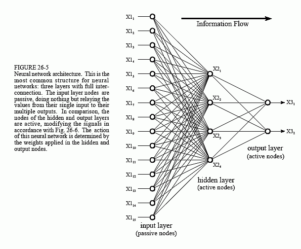
Many different neural network structures have been tried, some based on imitating what a biologist sees under the microscope, some based on a more mathematical analysis of the problem. The most commonly used structure is shown in Fig. 26-5. This neural network is formed in three layers, called the input layer, hidden layer, and output layer. Each layer consists of one or more nodes, represented in this diagram by the small circles. The lines between the nodes indicate the flow of information from one node to the next. In this particular type of neural network, the information flows only from the input to the output (that is, from left-to-right). Other types of neural networks have more intricate connections, such as feedback paths.
The nodes of the input layer are passive, meaning they do not modify the data. They receive a single value on their input, and duplicate the value to

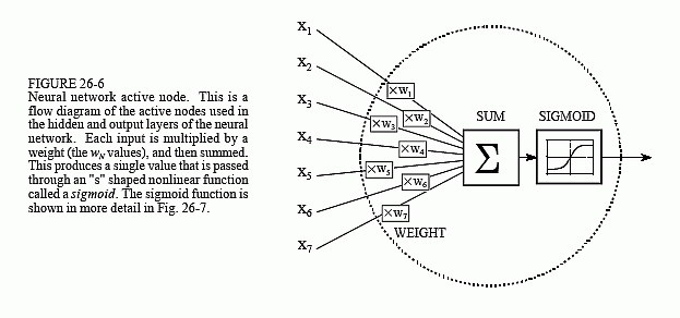
their multiple outputs. In comparison, the nodes of the hidden and output layer are active. This means they modify the data as shown in Fig. 26-6. The variables: X11,X12…X115 hold the data to be evaluated (see Fig. 26-5). For example, they may be pixel values from an image, samples from an audio signal, stock market prices on successive days, etc. They may also be the output of some other algorithm, such as the classifiers in our cancer detection example: diameter, brightness, edge sharpness, etc.
Each value from the input layer is duplicated and sent to all of the hidden nodes. This is called a fully interconnected structure. As shown in Fig. 26-6, the values entering a hidden node are multiplied by weights, a set of predetermined numbers stored in the program. The weighted inputs are then added to produce a single number. This is shown in the diagram by the symbol, ∑. Before leaving the node, this number is passed through a nonlinear mathematical function called a sigmoid. This is an "s" shaped curve that limits the node's output. That is, the input to the sigmoid is a value between -∞ and +∞, while its output can only be between 0 and 1.
The outputs from the hidden layer are represented in the flow diagram (Fig 26-5) by the variables: X21,X22,X23 and X24. Just as before, each of these values is duplicated and applied to the next layer. The active nodes of the output layer combine and modify the data to produce the two output values of this network, X31 and X32.
Neural networks can have any number of layers, and any number of nodes per layer. Most applications use the three layer structure with a maximum of a few hundred input nodes. The hidden layer is usually about 10% the size of the input layer. In the case of target detection, the output layer only needs a single node. The output of this node is thresholded to provide a positive or negative indication of the target's presence or absence in the input data.
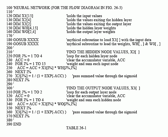
Table 26-1 is a program to carry out the flow diagram of Fig. 26-5. The key point is that this architecture is very simple and very generalized. This same flow diagram can be used for many problems, regardless of their particular quirks. The ability of the neural network to provide useful data manipulation lies in the proper selection of the weights. This is a dramatic departure from conventional information processing where solutions are described in step-by-step procedures.
As an example, imagine a neural network for recognizing objects in a sonar signal. Suppose that 1000 samples from the signal are stored in a computer. How does the computer determine if these data represent a submarine, whale, undersea mountain, or nothing at all? Conventional DSP would approach this problem with mathematics and algorithms, such as correlation and frequency spectrum analysis. With a neural network, the 1000 samples are simply fed into the input layer, resulting in values popping from the output layer. By selecting the proper weights, the output can be configured to report a wide range of information. For instance, there might be outputs for: submarine (yes/no), whale (yes/no), undersea mountain (yes/no), etc.

With other weights, the outputs might classify the objects as: metal or non-metal, biological or nonbiological, enemy or ally, etc. No algorithms, no rules, no procedures; only a relationship between the input and output dictated by the values of the weights selected.


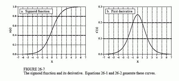
Figure 26-7a shows a closer look at the sigmoid function, mathematically described by the equation:

The exact shape of the sigmoid is not important, only that it is a smooth threshold. For comparison, a simple threshold produces a value of one when x > 0, and a value of zero when x < 0. The sigmoid performs this same basic thresholding function, but is also differentiable, as shown in Fig. 26-7b. While the derivative is not used in the flow diagram (Fig. 25-5), it is a critical part of finding the proper weights to use. More about this shortly. An advantage of the sigmoid is that there is a shortcut to calculating the value of its derivative:

For example, if x = 0, then s(x) = 0.5 (by Eq. 26-1), and the first derivative is calculated: s'(x) = 0.5(1 - 0.5) = 0.25. This isn't a critical concept, just a trick to make the algebra shorter.
Wouldn't the neural network be more flexible if the sigmoid could be adjusted left-or-right, making it centered on some other value than x = 0? The answer is yes, and most neural networks allow for this. It is very simple to implement; an additional node is added to the input layer, with its input always having a value of one. When this is multiplied by the weights of the hidden layer, it provides a bias (DC offset) to each sigmoid. This addition is called a bias node. It is treated the same as the other nodes, except for the constant input.
Can neural networks be made without a sigmoid or similar nonlinearity? To answer this, look at the three-layer network of Fig. 26-5. If the sigmoids were not present, the three layers would collapse into only two layers. In other words, the summations and weights of the hidden and output layers could be combined into a single layer, resulting in only a two-layer network.
