The Scientist and Engineer's Guide to
Digital Signal Processing
By Steven W. Smith, Ph.D.
Book Search
Table of contents
- 1: The Breadth and Depth of DSP
- 2: Statistics, Probability and Noise
- 3: ADC and DAC
- 4: DSP Software
- 5: Linear Systems
- 6: Convolution
- 7: Properties of Convolution
- 8: The Discrete Fourier Transform
- 9: Applications of the DFT
- 10: Fourier Transform Properties
- 11: Fourier Transform Pairs
- 12: The Fast Fourier Transform
- 13: Continuous Signal Processing
- 14: Introduction to Digital Filters
- 15: Moving Average Filters
- 16: Windowed-Sinc Filters
- 17: Custom Filters
- 18: FFT Convolution
- 19: Recursive Filters
- 20: Chebyshev Filters
- 21: Filter Comparison
- 22: Audio Processing
- 23: Image Formation & Display
- 24: Linear Image Processing
- 25: Special Imaging Techniques
- 26: Neural Networks (and more!)
- 27: Data Compression
- 28: Digital Signal Processors
- 29: Getting Started with DSPs
- 30: Complex Numbers
- 31: The Complex Fourier Transform
- 32: The Laplace Transform
- 33: The z-Transform
- 34: Explaining Benford's Law
How to order your own hardcover copy
Wouldn't you rather have a bound book instead of 640 loose pages?Your laser printer will thank you!
Order from Amazon.com.
Chapter 10: Fourier Transform Properties
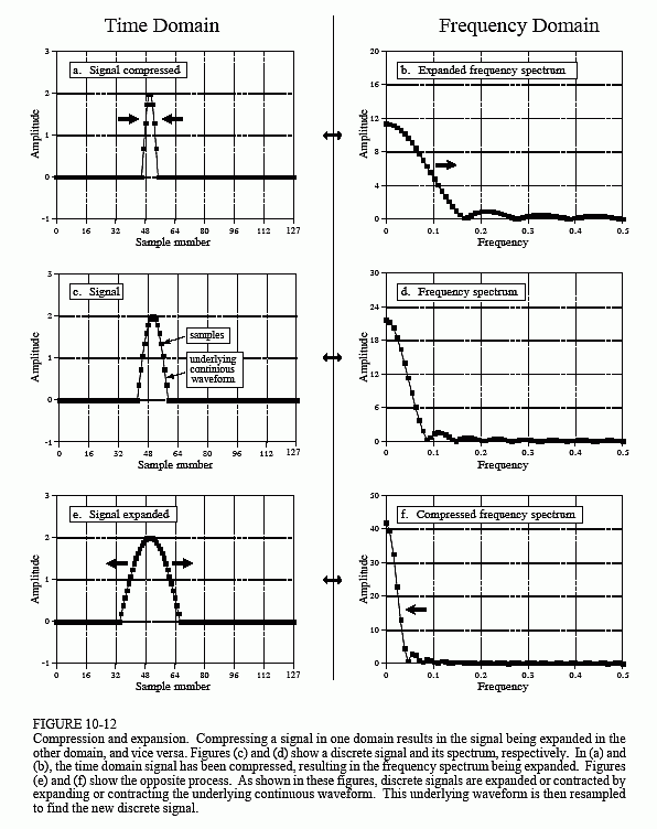
As shown in Fig. 10-12, a compression of the signal in one domain results in an expansion in the other, and vice versa. For continuous signals, if X(f) is the Fourier Transform of x(t), then 1/k × X(f/k) is the Fourier Transform of x(kt), where k is the parameter controlling the expansion or contraction. If an event happens faster (it is compressed in time), it must be composed of higher frequencies. If an event happens slower (it is expanded in time), it must be composed of lower frequencies. This pattern holds if taken to either of the two extremes. That is, if the time domain signal is compressed so far that it becomes an impulse, the corresponding frequency spectrum is expanded so far that it becomes a constant value. Likewise, if the time domain is expanded until it becomes a constant value, the frequency domain becomes an impulse.
Discrete signals behave in a similar fashion, but there are a few more details. The first issue with discrete signals is aliasing. Imagine that the

pulse in (a) is compressed several times more than is shown. The frequency spectrum is expanded by an equal factor, and several of the humps in (b) are pushed to frequencies beyond 0.5. The resulting aliasing breaks the simple expansion/contraction relationship. This type of aliasing can also happen in the time domain. Imagine that the frequency spectrum in (f) is compressed much harder, resulting in the time domain signal in (e) expanding into neighboring periods.
A second issue is to define exactly what it means to compress or expand a discrete signal. As shown in Fig. 10-12a, a discrete signal is compressed by compressing the underlying continuous curve that the samples lie on, and then resampling the new continuous curve to find the new discrete signal. Likewise, this same process for the expansion of discrete signals is shown in (e). When a discrete signal is compressed, events in the signal (such as the width of the pulse) happen over a fewer number of samples. Likewise, events in an expanded signal happen over a greater number of samples.
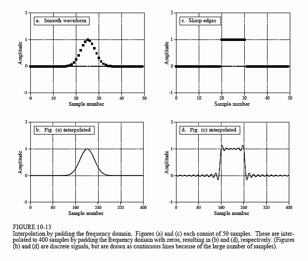
An equivalent way of looking at this procedure is to keep the underlying continuous waveform the same, but resample it at a different sampling rate. For instance, look at Fig. 10-13a, a discrete Gaussian waveform composed of 50 samples. In (b), the same underlying curve is represented by 400 samples. The change between (a) and (b) can be viewed in two ways: (1) the sampling rate has been kept constant, but the underlying waveform has been expanded to be eight times wider, or (2) the underlying waveform has been kept constant, but the sampling rate has increased by a factor of eight.
Methods for changing the sampling rate in this way are called multirate techniques. If more samples are added, it is called interpolation. If fewer samples are used to represent the signal, it is called decimation. Chapter 3 describes how multirate techniques are used in ADC and DAC.
Here is the problem: if we are given an arbitrary discrete signal, how do we know what the underlying continuous curve is? It depends on if the signal's information is encoded in the time domain or in the frequency domain. For time domain encoded signals, we want the underlying continious waveform to be a smooth curve that passes through all the samples. In the simplest case, we might drawing straight lines between the points and then round the rough corners. The next level of sophistication is to use a curve fitting algorithm, such as a spline function or polynomial fit. There is not a single "correct" answer to this problem. This approach is based on minimize irregularities in the time domain waveform, and completely ignores the freqeuncy domain.
When a signal has information encoded in the frequency domain, we ignore the time domain waveform and concentrate on the frequency spectrum. As discussed in the last chapter, a finer sampling of a frequency spectrum (more samples between frequency 0 and 0.5) can be obtained by padding the time domain signal with zeros before taking the DFT. Duality allows this to work in the opposite direction. If we want a finer sampling in the time domain (interpolation), pad the frequency spectrum with zeros before taking the Inverse DFT. Say we want to interpolate a 50 sample signal into a 400 sample signal. It's done like this: (1) Take the 50 samples and add zeros to make the signal 64 samples long. (2) Use a 64 point DFT to find the frequency spectrum, which will consist of a 33 point real part and a 33 point imaginary part. (3) Pad the right side of the frequency spectrum

(both the real and imaginary parts) with 224 zeros to make the frequency spectrum 257 points long. (4) Use a 512 point Inverse DFT to transform the data back into the time domain. This will result in a 512 sample signal that is a high resolution version of the 64 sample signal. The first 400 samples of this signal are an interpolated version of the original 50 samples.
The key feature of this technique is that the interpolated signal is composed of exactly the same frequencies as the original signal. This may or may not provide a well-behaved fit in the time domain. For example, Figs. 10-13 (a) and (b) show a 50 sample signal being interpolated into a 400 sample signal by this method. The interpolation is a smooth fit between the original points, much as if a curve fitting routine had been used. In comparison, (c) and (d) show another example where the time domain is a mess! The oscillatory behavior shown in (d) arises at edges or other discontinuities in the signal. This also includes any discontinuity between sample zero and N-1, since the time domain is viewed as being circular. This overshoot at discontinuities is called the Gibbs effect, and is discussed in Chapter 11. Another frequency domain interpolation technique is presented in Chapter 3, adding zeros between the time domain samples and low-pass filtering.
