The Scientist and Engineer's Guide to
Digital Signal Processing
By Steven W. Smith, Ph.D.
Book Search
Table of contents
- 1: The Breadth and Depth of DSP
- 2: Statistics, Probability and Noise
- 3: ADC and DAC
- 4: DSP Software
- 5: Linear Systems
- 6: Convolution
- 7: Properties of Convolution
- 8: The Discrete Fourier Transform
- 9: Applications of the DFT
- 10: Fourier Transform Properties
- 11: Fourier Transform Pairs
- 12: The Fast Fourier Transform
- 13: Continuous Signal Processing
- 14: Introduction to Digital Filters
- 15: Moving Average Filters
- 16: Windowed-Sinc Filters
- 17: Custom Filters
- 18: FFT Convolution
- 19: Recursive Filters
- 20: Chebyshev Filters
- 21: Filter Comparison
- 22: Audio Processing
- 23: Image Formation & Display
- 24: Linear Image Processing
- 25: Special Imaging Techniques
- 26: Neural Networks (and more!)
- 27: Data Compression
- 28: Digital Signal Processors
- 29: Getting Started with DSPs
- 30: Complex Numbers
- 31: The Complex Fourier Transform
- 32: The Laplace Transform
- 33: The z-Transform
- 34: Explaining Benford's Law
How to order your own hardcover copy
Wouldn't you rather have a bound book instead of 640 loose pages?Your laser printer will thank you!
Order from Amazon.com.
Chapter 14: Introduction to Digital Filters
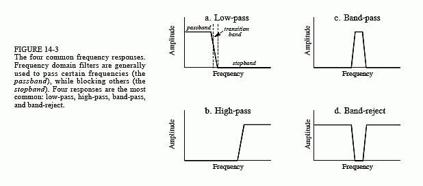
Figure 14-3 shows the four basic frequency responses. The purpose of these filters is to allow some frequencies to pass unaltered, while completely blocking other frequencies. The passband refers to those frequencies that are passed, while the stopband contains those frequencies that are blocked. The transition band is between. A fast roll-off means that the transition band is very narrow. The division between the passband and transition band is called the cutoff frequency. In analog filter design, the cutoff frequency is usually defined to be where the amplitude is reduced to 0.707 (i.e., -3dB). Digital filters are less standardized, and it is common to see 99%, 90%, 70.7%, and 50% amplitude levels defined to be the cutoff frequency.
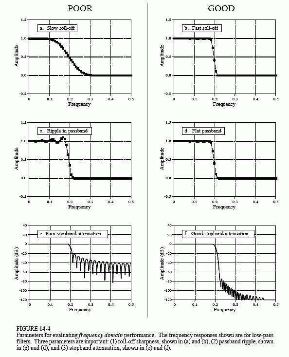
Figure 14-4 shows three parameters that measure how well a filter performs in the frequency domain. To separate closely spaced frequencies, the filter must have a fast roll-off, as illustrated in (a) and (b). For the passband frequencies to move through the filter unaltered, there must be no passband ripple, as shown in (c) and (d). Lastly, to adequately block the stopband frequencies, it is necessary to have good stopband attenuation, displayed in (e) and (f).


Why is there nothing about the phase in these parameters? First, the phase isn't important in most frequency domain applications. For example, the phase of an audio signal is almost completely random, and contains little useful information. Second, if the phase is important, it is very easy to make digital filters with a perfect phase response, i.e., all frequencies pass through the filter with a zero phase shift (also discussed in Chapter 19). In comparison, analog filters are ghastly in this respect.
Previous chapters have described how the DFT converts a system's impulse response into its frequency response. Here is a brief review. The quickest
way to calculate the DFT is by means of the FFT algorithm presented in Chapter 12. Starting with a filter kernel N samples long, the FFT calculates the frequency spectrum consisting of an N point real part and an N point imaginary part. Only samples 0 to N/2 of the FFT's real and imaginary parts contain useful information; the remaining points are duplicates (negative frequencies) and can be ignored. Since the real and imaginary parts are difficult for humans to understand, they are usually converted into polar notation as described in Chapter 8. This provides the magnitude and phase signals, each running from sample 0 to sample N/2 (i.e., N/2 + 1 samples in each signal). For example, an impulse response of 256 points will result in a frequency response running from point 0 to 128. Sample 0 represents DC, i.e., zero frequency. Sample 128 represents one-half of the sampling rate. Remember, no frequencies higher than one-half of the sampling rate can appear in sampled data.
The number of samples used to represent the impulse response can be arbitrarily large. For instance, suppose you want to find the frequency response of a filter kernel that consists of 80 points. Since the FFT only works with signals that are a power of two, you need to add 48 zeros to the signal to bring it to a length of 128 samples. This padding with zeros does not change the impulse response. To understand why this is so, think about what happens to these added zeros when the input signal is convolved with the system's impulse response. The added zeros simply vanish in the convolution, and do not affect the outcome.
Taking this a step further, you could add many zeros to the impulse response to make it, say, 256, 512, or 1024 points long. The important idea is that longer impulse responses result in a closer spacing of the data points in the frequency response. That is, there are more samples spread between DC and one-half of the sampling rate. Taking this to the extreme, if the impulse response is padded with an infinite number of zeros, the data points in the frequency response are infinitesimally close together, i.e., a continuous line. In other words, the frequency response of a filter is really a continuous signal between DC and one-half of the sampling rate. The output of the DFT is a sampling of this continuous line. What length of impulse response should you use when calculating a filter's frequency response? As a first thought, try , but don't be afraid to change it if needed (such as insufficient resolution or excessive computation time).
Keep in mind that the "good" and "bad" parameters discussed in this chapter are only generalizations. Many signals don't fall neatly into categories. For example, consider an EKG signal contaminated with 60 hertz interference. The information is encoded in the time domain, but the interference is best dealt with in the frequency domain. The best design for this application is

bound to have trade-offs, and might go against the conventional wisdom of this chapter. Remember the number one rule of education: A paragraph in a book doesn't give you a license to stop thinking.
