The Scientist and Engineer's Guide to
Digital Signal Processing
By Steven W. Smith, Ph.D.
Book Search
Table of contents
- 1: The Breadth and Depth of DSP
- 2: Statistics, Probability and Noise
- 3: ADC and DAC
- 4: DSP Software
- 5: Linear Systems
- 6: Convolution
- 7: Properties of Convolution
- 8: The Discrete Fourier Transform
- 9: Applications of the DFT
- 10: Fourier Transform Properties
- 11: Fourier Transform Pairs
- 12: The Fast Fourier Transform
- 13: Continuous Signal Processing
- 14: Introduction to Digital Filters
- 15: Moving Average Filters
- 16: Windowed-Sinc Filters
- 17: Custom Filters
- 18: FFT Convolution
- 19: Recursive Filters
- 20: Chebyshev Filters
- 21: Filter Comparison
- 22: Audio Processing
- 23: Image Formation & Display
- 24: Linear Image Processing
- 25: Special Imaging Techniques
- 26: Neural Networks (and more!)
- 27: Data Compression
- 28: Digital Signal Processors
- 29: Getting Started with DSPs
- 30: Complex Numbers
- 31: The Complex Fourier Transform
- 32: The Laplace Transform
- 33: The z-Transform
- 34: Explaining Benford's Law
How to order your own hardcover copy
Wouldn't you rather have a bound book instead of 640 loose pages?Your laser printer will thank you!
Order from Amazon.com.
Chapter 2: Statistics, Probability and Noise
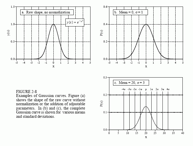
Signals formed from random processes usually have a bell shaped pdf. This is called a normal distribution, a Gauss distribution, or a Gaussian, after the great German mathematician, Karl Friedrich Gauss (1777-1855). The reason why this curve occurs so frequently in nature will be discussed shortly in conjunction with digital noise generation. The basic shape of the curve is generated from a negative squared exponent:
This raw curve can be converted into the complete Gaussian by adding an adjustable mean, ?, and standard deviation, σ. In addition, the equation must be normalized so that the total area under the curve is equal to one, a requirement of all probability distribution functions. This results in the general form of the normal distribution, one of the most important relations in statistics and probability:

Figure 2-8 shows several examples of Gaussian curves with various means and standard deviations. The mean centers the curve over a particular value, while the standard deviation controls the width of the bell shape.
An interesting characteristic of the Gaussian is that the tails drop toward zero very rapidly, much faster than with other common functions such as decaying exponentials or 1/x. For example, at two, four, and six standard

deviations from the mean, the value of the Gaussian curve has dropped to about 1/19, 1/7563, and 1/166,666,666, respectively. This is why normally distributed signals, such as illustrated in Fig. 2-6c, appear to have an approximate peak-to-peak value. In principle, signals of this type can experience excursions of unlimited amplitude. In practice, the sharp drop of the Gaussian pdf dictates that these extremes almost never occur. This results in the waveform having a relatively bounded appearance with an apparent peakto- peak amplitude of about 6-8σ.
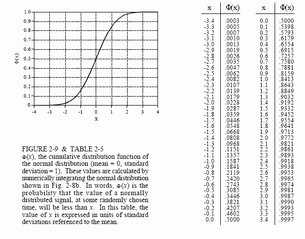
As previously shown, the integral of the pdf is used to find the probability that a signal will be within a certain range of values. This makes the integral of the pdf important enough that it is given its own name, the cumulative distribution function (cdf). An especially obnoxious problem with the Gaussian is that it cannot be integrated using elementary methods. To get around this, the integral of the Gaussian can be calculated by numerical integration. This involves sampling the continuous Gaussian curve very finely, say, a few million points between -10σ and +10σ. The samples in this discrete signal are then added to simulate integration. The discrete curve resulting from this simulated integration is then stored in a table for use in calculating probabilities.
The cdf of the normal distribution is shown in Fig. 2-9, with its numeric values listed in Table 2-5. Since this curve is used so frequently in probability, it is given its own symbol: Φ(x) (upper case Greek phi). For example, Φ(-2) has a value of 0.0228. This indicates that there is a 2.28% probability that the value of the signal will be between -∞ and two standard deviations below the mean, at any randomly chosen time. Likewise, the value: Φ(1) = 0.8413, means there is an 84.13% chance that the value of the signal, at a randomly selected instant, will be between -∞ and one standard deviation above the mean. To calculate the probability that the signal will be will be between two values, it is necessary to subtract the appropriate numbers found in the Φ(x) table. For example, the probability that the value of the signal, at some randomly chosen time, will be between two standard deviations below the mean and one standard deviation above the mean, is given by: Φ(1) - Φ(-2) = 0.8185 or 81.85%
Using this method, samples taken from a normally distributed signal will be within ?1σ of the mean about 68% of the time. They will be within ?2σ about 95% of the time, and within ?3σ about 99.75% of the time. The probability of the signal being more than 10 standard deviations from the mean is so minuscule, it would be expected to occur for only a few microseconds since the beginning of the universe, about 10 billion years!
Equation 2-8 can also be used to express the probability mass function of normally distributed discrete signals. In this case, x is restricted to be one of the quantized levels that the signal can take on, such as one of the 4096 binary values exiting a 12 bit analog-to-digital converter. Ignore the 1/ √2πσ term, it is only used to make the total area under the pdf curve equal to one. Instead, you must include whatever term is needed to make the sum of all the values in the pmf equal to one. In most cases, this is done by

generating the curve without worrying about normalization, summing all of the unnormalized values, and then dividing all of the values by the sum.
