The Scientist and Engineer's Guide to
Digital Signal Processing
By Steven W. Smith, Ph.D.
Book Search

Table of contents
- 1: The Breadth and Depth of DSP
- 2: Statistics, Probability and Noise
- 3: ADC and DAC
- 4: DSP Software
- 5: Linear Systems
- 6: Convolution
- 7: Properties of Convolution
- 8: The Discrete Fourier Transform
- 9: Applications of the DFT
- 10: Fourier Transform Properties
- 11: Fourier Transform Pairs
- 12: The Fast Fourier Transform
- 13: Continuous Signal Processing
- 14: Introduction to Digital Filters
- 15: Moving Average Filters
- 16: Windowed-Sinc Filters
- 17: Custom Filters
- 18: FFT Convolution
- 19: Recursive Filters
- 20: Chebyshev Filters
- 21: Filter Comparison
- 22: Audio Processing
- 23: Image Formation & Display
- 24: Linear Image Processing
- 25: Special Imaging Techniques
- 26: Neural Networks (and more!)
- 27: Data Compression
- 28: Digital Signal Processors
- 29: Getting Started with DSPs
- 30: Complex Numbers
- 31: The Complex Fourier Transform
- 32: The Laplace Transform
- 33: The z-Transform
- 34: Explaining Benford's Law
How to order your own hardcover copy
Wouldn't you rather have a bound book instead of 640 loose pages?Your laser printer will thank you!
Order from Amazon.com.
Chapter 18: FFT Convolution
FFT convolution uses the principle that multiplication in the frequency domain corresponds to convolution in the time domain. The input signal is transformed into the frequency domain using the DFT, multiplied by the frequency response of the filter, and then transformed back into the time domain using the Inverse DFT. This basic technique was known since the days of Fourier; however, no one really cared. This is because the time required to calculate the DFT was longer than the time to directly calculate the convolution. This changed in 1965 with the development of the Fast Fourier Transform (FFT). By using the FFT algorithm to calculate the DFT, convolution via the frequency domain can be faster than directly convolving the time domain signals. The final result is the same; only the number of calculations has been changed by a more efficient algorithm. For this reason, FFT convolution is also called high-speed convolution.
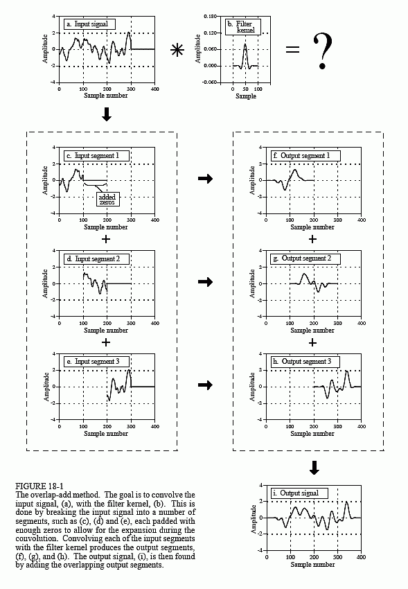
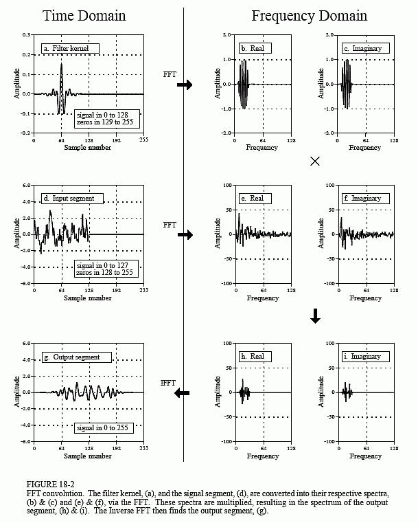
FFT convolution uses the overlap-add method shown in Fig. 18-1; only the way that the input segments are converted into the output segments is changed. Figure 18-2 shows an example of how an input segment is converted into an output segment by FFT convolution. To start, the frequency response of the filter is found by taking the DFT of the filter kernel, using the FFT. For instance, (a) shows an example filter kernel, a windowed-sinc band-pass filter. The FFT converts this into the real and imaginary parts of the frequency response, shown in (b) & (c). These frequency domain signals may not look like a band-pass filter because they are in rectangular form. Remember, polar form is usually best for humans to understand the frequency domain, while rectangular form is normally best for mathematical calculations. These real and imaginary parts are stored in the computer for use when each segment is being calculated.
Figure (d) shows the input segment to being processed. The FFT is used to find its frequency spectrum, shown in (e) & (f). The frequency spectrum of the output segment, (h) & (i) is then found by multiplying the filter's frequency response, (b) & (c), by the spectrum of the input segment, (e) & (f). Since these spectra consist of real and imaginary parts, they are multiplied according to Eq. 9-1 in Chapter 9. The Inverse FFT is then used to find the output segment, (g), from its frequency spectrum, (h) & (i). It is important to recognize that this output segment is exactly the same as would be obtained by the direct convolution of the input segment, (d), and the filter kernel, (a).
The FFTs must be long enough that circular convolution does not take place (also described in Chapter 9). This means that the FFT should be the same length as the output segment, (g). For instance, in the example of Fig. 18-2, the filter kernel contains 129 points and each segment contains 128 points, making output segment 256 points long. This calls for 256 point FFTs to be used. This means that the filter kernel, (a), must be padded with 127 zeros to bring it to a total length of 256 points. Likewise, each of the input segments, (d), must be padded with 128 zeros. As another example, imagine you need to convolve a very long signal with a filter kernel having 600 samples. One alternative would be to use segments of 425 points, and 1024 point FFTs. Another alternative would be to use segments of 1449 points, and 2048 point FFTs.
Table 18-1 shows an example program to carry out FFT convolution. This program filters a 10 million point signal by convolving it with a 400 point filter kernel. This is done by breaking the input signal into 16000 segments, with each segment having 625 points. When each of these segments is convolved with the filter kernel, an output segment of 625 + 400 - 1 = 1024 points is produced. Thus, 1024 point FFTs are used. After defining and initializing all the arrays (lines 130 to 230), the first step is to calculate and store the frequency response of the filter (lines 250 to 310). Line 260 calls a mythical subroutine that loads the filter kernel into XX[0] through XX[399], and sets XX[400] through XX[1023] to a value of zero. The subroutine in line 270 is the FFT, transforming the 1024 samples held in XX[ ] into the 513 samples held in REX[ ] & IMX[ ], the real and
imaginary parts of the frequency response. These values are transferred into the arrays REFR[ ] & IMFR[ ] (for: REal and IMaginary Frequency Response), to be used later in the program.
The FOR-NEXT loop between lines 340 and 580 controls how the 16000 segments are processed. In line 360, a subroutine loads the next segment to be processed into XX[0] through XX[624], and sets XX[625] through XX[1023] to a value of zero. In line 370, the FFT subroutine is used to find this segment's frequency spectrum, with the real part being placed in the 513 points of REX[ ], and the imaginary part being placed in the 513 points of IMX[ ]. Lines 390 to 430 show the multiplication of the segment's frequency spectrum, held in REX[ ] & IMX[ ], by the filter's frequency response, held in REFR[ ] and IMFR[ ]. The result of the multiplication is stored in REX[ ] & IMX[ ], overwriting the data previously there. Since this is now the frequency spectrum of the output segment, the IFFT can be used to find the output segment. This is done by the mythical IFFT subroutine in line 450, which transforms the 513 points held in REX[ ] & IMX[ ] into the 1024 points held in XX[ ], the output segment.
Lines 470 to 550 handle the overlapping of the segments. Each output segment is divided into two sections. The first 625 points (0 to 624) need to be combined with the overlap from the previous output segment, and then written to the output signal. The last 399 points (625 to 1023) need to be saved so that they can overlap with the next output segment.
To understand this, look back at Fig 18-1. Samples 100 to 199 in (g) need to be combined with the overlap from the previous output segment, (f), and can then be moved to the output signal (i). In comparison, samples 200 to 299 in (g) need to be saved so that they can be combined with the next output segment, (h).
Now back to the program. The array OLAP[ ] is used to hold the 399 samples that overlap from one segment to the next. In lines 470 to 490 the 399 values in this array (from the previous output segment) are added to the output segment currently being worked on, held in XX[ ]. The mythical subroutine in line 550 then outputs the 625 samples in XX[0] to XX[624] to the file holding the output signal. The 399 samples of the current output segment that need to be held over to the next output segment are then stored in OLAP[ ] in lines 510 to 530.
After all 0 to 15999 segments have been processed, the array, OLAP[ ], will contain the 399 samples from segment 15999 that should overlap segment 16000. Since segment 16000 doesn't exist (or can be viewed as containing all zeros), the 399 samples are written to the output signal in line 600. This makes the length of the output signal points. This matches the length of input signal, plus the length of the filter kernel, minus 1.