The Scientist and Engineer's Guide to
Digital Signal Processing
By Steven W. Smith, Ph.D.
Book Search

Table of contents
- 1: The Breadth and Depth of DSP
- 2: Statistics, Probability and Noise
- 3: ADC and DAC
- 4: DSP Software
- 5: Linear Systems
- 6: Convolution
- 7: Properties of Convolution
- 8: The Discrete Fourier Transform
- 9: Applications of the DFT
- 10: Fourier Transform Properties
- 11: Fourier Transform Pairs
- 12: The Fast Fourier Transform
- 13: Continuous Signal Processing
- 14: Introduction to Digital Filters
- 15: Moving Average Filters
- 16: Windowed-Sinc Filters
- 17: Custom Filters
- 18: FFT Convolution
- 19: Recursive Filters
- 20: Chebyshev Filters
- 21: Filter Comparison
- 22: Audio Processing
- 23: Image Formation & Display
- 24: Linear Image Processing
- 25: Special Imaging Techniques
- 26: Neural Networks (and more!)
- 27: Data Compression
- 28: Digital Signal Processors
- 29: Getting Started with DSPs
- 30: Complex Numbers
- 31: The Complex Fourier Transform
- 32: The Laplace Transform
- 33: The z-Transform
- 34: Explaining Benford's Law
How to order your own hardcover copy
Wouldn't you rather have a bound book instead of 640 loose pages?Your laser printer will thank you!
Order from Amazon.com.
Chapter 24: Linear Image Processing
Figure 24-4 shows several 3×3 operations. Figure (a) is an image acquired by an airport x-ray baggage scanner. When this image is convolved with a 3×3 delta function (a one surrounded by 8 zeros), the image remains unchanged. While this is not interesting by itself, it forms the baseline for the other filter kernels.
Figure (b) shows the image convolved with a 3×3 kernel consisting of a one, a negative one, and 7 zeros. This is called the shift and subtract operation, because a shifted version of the image (corresponding to the -1) is subtracted from the original image (corresponding to the 1). This processing produces the optical illusion that some objects are closer or farther away than the background, making a 3D or embossed effect. The brain interprets images as if the lighting is from above, the normal way the world presents itself. If the edges of an object are bright on the top and dark on the bottom, the object is perceived to be poking out from the background. To see another interesting effect, turn the picture upside down, and the objects will be pushed into the background.
Figure (c) shows an edge detection PSF, and the resulting image. Every edge in the original image is transformed into narrow dark and light bands that run parallel to the original edge. Thresholding this image can isolate either the dark or light band, providing a simple algorithm for detecting the edges in an image.
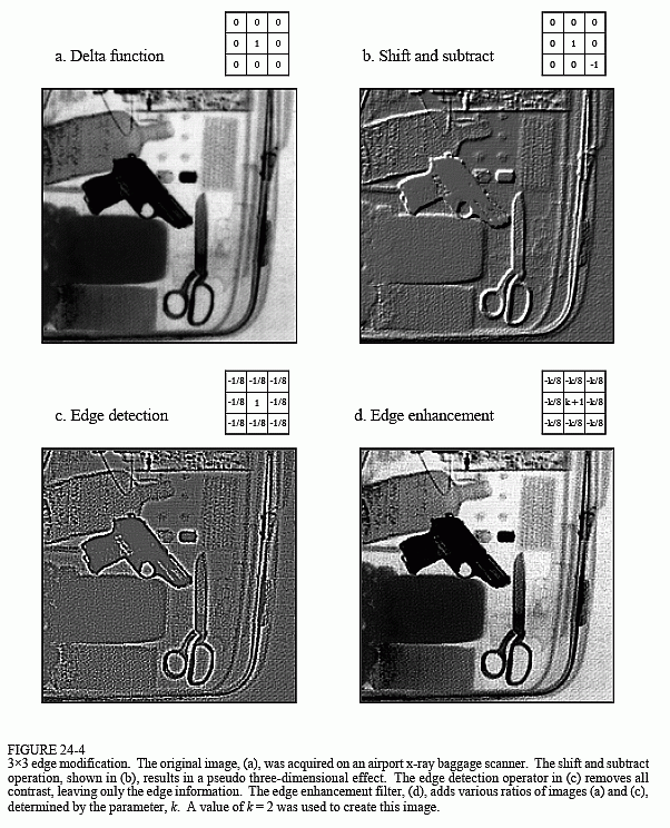
A common image processing technique is shown in (d): edge enhancement. This is sometimes called a sharpening operation. In (a), the objects have good contrast (an appropriate level of darkness and lightness) but very blurry edges. In (c), the objects have absolutely no contrast, but very sharp edges. The strategy is to multiply the image with good edges by a constant, k, and add it to the image with good contrast. This is equivalent to convolving the original image with the 3×3 PSF shown in (d). If k is set to 0, the PSF becomes a delta function, and the image is left unchanged. As k is made larger, the image shows better edge definition. For the image in (d), a value of k = 2 was used: two parts of image (c) to one part of image (a). This operation mimics the eye's ability to sharpen edges, allowing objects to be more easily separated from the background.
Convolution with any of these PSFs can result in negative pixel values appearing in the final image. Even if the program can handle negative values for pixels, the image display cannot. The most common way around this is to add an offset to each of the calculated pixels, as is done in these images. An alternative is to truncate out-of-range values.