The Scientist and Engineer's Guide to
Digital Signal Processing
By Steven W. Smith, Ph.D.
Book Search
Table of contents
- 1: The Breadth and Depth of DSP
- 2: Statistics, Probability and Noise
- 3: ADC and DAC
- 4: DSP Software
- 5: Linear Systems
- 6: Convolution
- 7: Properties of Convolution
- 8: The Discrete Fourier Transform
- 9: Applications of the DFT
- 10: Fourier Transform Properties
- 11: Fourier Transform Pairs
- 12: The Fast Fourier Transform
- 13: Continuous Signal Processing
- 14: Introduction to Digital Filters
- 15: Moving Average Filters
- 16: Windowed-Sinc Filters
- 17: Custom Filters
- 18: FFT Convolution
- 19: Recursive Filters
- 20: Chebyshev Filters
- 21: Filter Comparison
- 22: Audio Processing
- 23: Image Formation & Display
- 24: Linear Image Processing
- 25: Special Imaging Techniques
- 26: Neural Networks (and more!)
- 27: Data Compression
- 28: Digital Signal Processors
- 29: Getting Started with DSPs
- 30: Complex Numbers
- 31: The Complex Fourier Transform
- 32: The Laplace Transform
- 33: The z-Transform
- 34: Explaining Benford's Law
How to order your own hardcover copy
Wouldn't you rather have a bound book instead of 640 loose pages?Your laser printer will thank you!
Order from Amazon.com.
Chapter 2: Statistics, Probability and Noise
Suppose we attach an 8 bit analog-to-digital converter to a computer, and acquire 256,000 samples of some signal. As an example, Fig. 2-4a shows 128 samples that might be a part of this data set. The value of each sample will be one of 256 possibilities, 0 through 255. The histogram displays the number of samples there are in the signal that have each of these possible values. Figure (b) shows the histogram for the 128 samples in (a). For
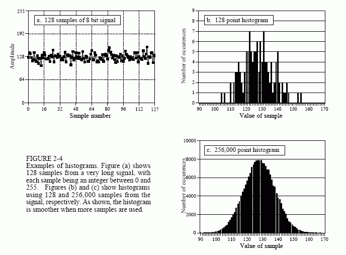
example, there are 2 samples that have a value of 110, 8 samples that have a value of 131, 0 samples that have a value of 170, etc. We will represent the histogram by Hi, where i is an index that runs from 0 to M-1, and M is the number of possible values that each sample can take on. For instance, H50 is the number of samples that have a value of 50. Figure (c) shows the histogram of the signal using the full data set, all 256k points. As can be seen, the larger number of samples results in a much smoother appearance. Just as with the mean, the statistical noise (roughness) of the histogram is inversely proportional to the square root of the number of samples used.
From the way it is defined, the sum of all of the values in the histogram must be equal to the number of points in the signal:

The histogram can be used to efficiently calculate the mean and standard deviation of very large data sets. This is especially important for images, which can contain millions of samples. The histogram groups samples together that have the same value. This allows the statistics to be calculated by working with a few groups, rather than a large number of individual samples. Using this approach, the mean and standard deviation are calculated from the histogram by the equations:


Table 2-3 contains a program for calculating the histogram, mean, and standard deviation using these equations. Calculation of the histogram is very fast, since it only requires indexing and incrementing. In comparison,

calculating the mean and standard deviation requires the time consuming operations of addition and multiplication. The strategy of this algorithm is to use these slow operations only on the few numbers in the histogram, not the many samples in the signal. This makes the algorithm much faster than the previously described methods. Think a factor of ten for very long signals with the calculations being performed on a general purpose computer.
The notion that the acquired signal is a noisy version of the underlying process is very important; so important that some of the concepts are given different names. The histogram is what is formed from an acquired signal. The corresponding curve for the underlying process is called the probability mass function (pmf). A histogram is always calculated using a finite number of samples, while the pmf is what would be obtained with an infinite number of samples. The pmf can be estimated (inferred) from the histogram, or it may be deduced by some mathematical technique, such as in the coin flipping example.
Figure 2-5 shows an example pmf, and one of the possible histograms that could be associated with it. The key to understanding these concepts rests in the units of the vertical axis. As previously described, the vertical axis of the histogram is the number of times that a particular value occurs in the signal. The vertical axis of the pmf contains similar information, except expressed on a fractional basis. In other words, each value in the histogram is divided by the total number of samples to approximate the pmf. This means that each value in the pmf must be between zero and one, and that the sum of all of the values in the pmf will be equal to one.
The pmf is important because it describes the probability that a certain value will be generated. For example, imagine a signal generated by the process described by Fig. 2-5b, such as previously shown in Fig. 2-4a. What is the probability that a sample taken from this signal will have a value of 120? Figure 2-5b provides the answer, 0.03, or about 1 chance in 34. What is the probability that a randomly chosen sample will have a value greater than 150? Adding up the values in the pmf for: 151, 152, 153,⋅⋅⋅, 255, provides the answer, 0.0122, or about 1 chance in 82. Thus, the signal would be expected to have a value exceeding 150 on an average of every 82 points. What is the probability that any one sample will be between 0 to 255? Summing all of the values in the histogram produces the probability of 1.00, a certainty that this will occur.
The histogram and pmf can only be used with discrete data, such as a digitized signal residing in a computer. A similar concept applies to continuous signals, such as voltages appearing in analog electronics. The probability density function (pdf), also called the probability distribution function, is to continuous signals what the probability mass function is to discrete signals. For example, imagine an analog signal passing through an analog-to-digital converter, resulting in the digitized signal of Fig. 2-4a. For simplicity, we will assume that voltages between 0 and 255 millivolts become digitized into digital numbers between 0 and 255. The pmf of this digital
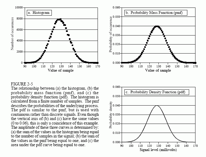
signal is shown by the markers in Fig. 2-5b. Similarly, the pdf of the analog signal is shown by the continuous line in (c), indicating the signal can take on a continuous range of values, such as the voltage in an electronic circuit.
The vertical axis of the pdf is in units of probability density, rather than just probability. For example, a pdf of 0.03 at 120.5 does not mean that the a voltage of 120.5 millivolts will occur 3% of the time. In fact, the probability of the continuous signal being exactly 120.5 millivolts is infinitesimally small. This is because there are an infinite number of possible values that the signal needs to divide its time between: 120.49997, 120.49998, 120.49999, etc. The chance that the signal happens to be exactly 120.50000⋅⋅⋅ is very remote indeed!
To calculate a probability, the probability density is multiplied by a range of values. For example, the probability that the signal, at any given instant, will be between the values of 120 and 121 is: (121 - 120) x 0.03 = 0.03. The probability that the signal will be between 120.4 and 120.5 is: (120.5 - 120.4) x 0.03 = 0.003, etc. If the pdf is not constant over the range of interest, the multiplication becomes the integral of the pdf over that range. In other words, the area under the pdf bounded by the specified values. Since the value of the signal must always be something, the total area under the pdf curve, the integral from -∞ to +∞, will always be equal to one. This is analogous to the sum of all of the pmf values being equal to one, and the sum of all of the histogram values being equal to N.
The histogram, pmf, and pdf are very similar concepts. Mathematicians always keep them straight, but you will frequently find them used interchangeably (and therefore, incorrectly) by many scientists and
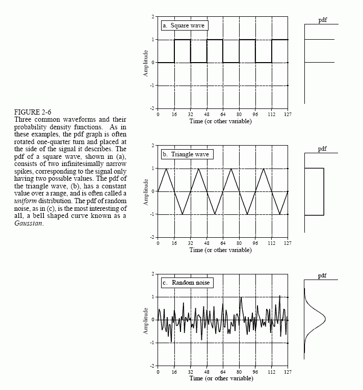
engineers. Figure 2-6 shows three continuous waveforms and their pdfs. If these were discrete signals, signified by changing the horizontal axis labeling to "sample number", pmfs would be used.
A problem occurs in calculating the histogram when the number of levels each sample can take on is much larger than the number of samples in the signal. This is always true for signals represented in floating point notation, where each sample is stored as a fractional value. For example, integer representation might require the sample value to be 3 or 4, while floating point allows millions of possible fractional values between 3 and 4. The previously described approach for calculating the histogram involves counting the number of samples that have each of the possible quantization levels. This is not possible with floating point data because there are billions of possible levels that would have to be taken into account. Even worse, nearly all of these possible levels would have no samples that correspond to them. For example, imagine a 10,000 sample signal, with each sample having one billion possible values. The conventional histogram would consist of one billion data points, with all but about 10,000 of them having a value of zero.
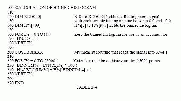
The solution to these problems is a technique called binning. This is done by arbitrarily selecting the length of the histogram to be some convenient number, such as 1000 points, often called bins. The value of each bin represent the total number of samples in the signal that have a value within a certain range. For example, imagine a floating point signal that contains values from 0.0 to 10.0, and a histogram with 1000 bins. Bin 0 in the histogram is the number of samples in the signal with a value between 0 and 0.01, bin 1 is the number of samples with a value between 0.01 and 0.02, and so forth, up to bin 999 containing the number of samples with a value between 9.99 and 10.0. Table 2-4 presents a program for calculating a binned histogram in this manner.
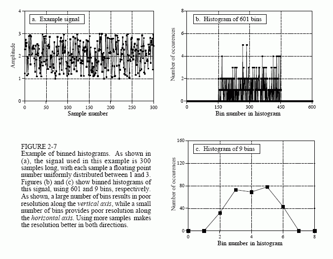
How many bins should be used? This is a compromise between two problems. As shown in Fig. 2-7, too many bins makes it difficult to estimate the amplitude of the underlying pmf. This is because only a few samples fall into each bin, making the statistical noise very high. At the other extreme, too few of bins makes it difficult to estimate the underlying pmf in the horizontal direction. In other words, the number of bins controls a tradeoff between resolution in along the y-axis, and resolution along the x-axis.
