The Scientist and Engineer's Guide to
Digital Signal Processing
By Steven W. Smith, Ph.D.
Book Search

Table of contents
- 1: The Breadth and Depth of DSP
- 2: Statistics, Probability and Noise
- 3: ADC and DAC
- 4: DSP Software
- 5: Linear Systems
- 6: Convolution
- 7: Properties of Convolution
- 8: The Discrete Fourier Transform
- 9: Applications of the DFT
- 10: Fourier Transform Properties
- 11: Fourier Transform Pairs
- 12: The Fast Fourier Transform
- 13: Continuous Signal Processing
- 14: Introduction to Digital Filters
- 15: Moving Average Filters
- 16: Windowed-Sinc Filters
- 17: Custom Filters
- 18: FFT Convolution
- 19: Recursive Filters
- 20: Chebyshev Filters
- 21: Filter Comparison
- 22: Audio Processing
- 23: Image Formation & Display
- 24: Linear Image Processing
- 25: Special Imaging Techniques
- 26: Neural Networks (and more!)
- 27: Data Compression
- 28: Digital Signal Processors
- 29: Getting Started with DSPs
- 30: Complex Numbers
- 31: The Complex Fourier Transform
- 32: The Laplace Transform
- 33: The z-Transform
- 34: Explaining Benford's Law
How to order your own hardcover copy
Wouldn't you rather have a bound book instead of 640 loose pages?Your laser printer will thank you!
Order from Amazon.com.
Chapter 5: Linear Systems
Keep in mind that the goal of this method is to replace a complicated problem with several easy ones. If the decomposition doesn't simplify the situation in some way, then nothing has been gained. There are two main ways to decompose signals in signal processing: impulse decomposition and Fourier decomposition. There are described in detail in the next several chapters. In addition, several minor decompositions are occasionally used. Here are brief descriptions of the two major decompositions, along with three minor ones.
Impulse Decomposition
As shown in Fig. 5-12, impulse decomposition breaks an N samples signal into
N component signals, each containing N samples. Each of the component
signals contains one point from the original signal, with the remainder of the
values being zero. A single nonzero point in a string of zeros is called an
impulse. Impulse decomposition is important because it allows signals to be
examined one sample at a time. Similarly, systems are characterized by how
they respond to impulses. By knowing how a system responds to an impulse,
the system's output can be calculated for any given input. This approach is
called convolution, and is the topic of the next two chapters.
Step Decomposition
Step decomposition, shown in Fig. 5-13, also breaks an N sample signal into N
component signals, each composed of N samples. Each component signal is a
step, that is, the first samples have a value of zero, while the last samples are
some constant value. Consider the decomposition of an N point signal, x[n],
into the components: x0[n], x1[n], x2[n], …, xN-1[n]. The kth component signal,
xk[n], is composed of zeros for points 0 through k - 1, while the remaining points have a value of: x[k] - x[k-1]. For example, the 5th component signal, x5[n], is composed of zeros for points 0 through 4, while the remaining samples have a value of: x[5] - x[4] (the difference between
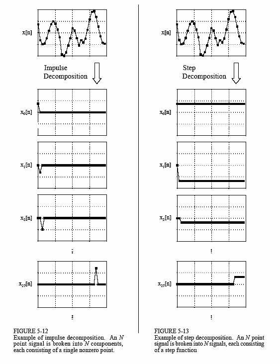
sample 4 and 5 of the original signal). As a special case, x0[n] has all of its samples equal to x[0]. Just as impulse decomposition looks at signals one point at a time, step decomposition characterizes signals by the difference between adjacent samples. Likewise, systems are characterized by how they respond to a change in the input signal.
Even/Odd Decomposition
The even/odd decomposition, shown in Fig. 5-14, breaks a signal into two
component signals, one having even symmetry and the other having odd
symmetry. An N point signal is said to have even symmetry if it is a mirror
image around point N/2. That is, sample x[N/2 + 1] must equal x[N/2 - 1],
sample x[N/2 + 2] must equal x[N/2 - 2], etc. Similarly, odd symmetry occurs
when the matching points have equal magnitudes but are opposite in sign, such
as: x[N/2 + 1] = -x[N/2 - 1], x[N/2 + 2] = -x[N/2 - 2], etc. These definitions assume that the signal is composed of an even number of samples, and that the
indexes run from 0 to N-1. The decomposition is calculated form the relations:

This may seem a strange definition of left-right symmetry, since N/2 - ½ (between two samples) is the exact center of the signal, not N/2. Likewise, this off-center symmetry means that sample zero needs special handling. What's this all about?
This decomposition is part of an important concept in DSP called circular symmetry. It is based on viewing the end of the signal as connected to the beginning of the signal. Just as point x[4] is next to point x[5], point x[N-1] is next to point x[0]. Picture a snake biting its own tail. When even and odd signals are viewed in this circular manner, there are actually two lines of symmetry, one at point x[N/2] and another at point x[0]. For example, in an even signal, this symmetry around x[0] means that point x[1] equals point x[N-1], point x[2] equals point x[N-2], etc. In an odd signal, point 0 and point N/2 always have a value of zero. In an even signal, point 0 and point N/2 are equal to the corresponding points in the original signal.
What is the motivation for viewing the last sample in a signal as being next to the first sample? There is nothing in conventional data acquisition to support this circular notion. In fact, the first and last samples generally have less in common than any other two points in the sequence. It's common sense! The missing piece to this puzzle is a DSP technique called Fourier analysis. The mathematics of Fourier analysis inherently views the signal as being circular, although it usually has no physical meaning in terms of where the data came from. We will look at this in more detail in Chapter 10. For now, the important thing to understand is that Eq. 5-1 provides a valid decomposition, simply because the even and odd parts can be added together to reconstruct the original signal.
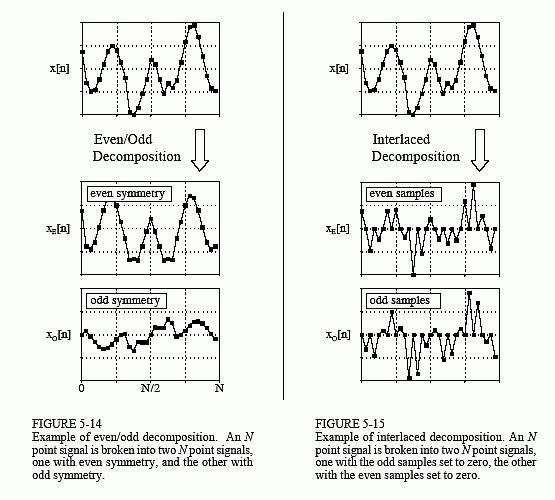
Interlaced Decomposition
As shown in Fig. 5-15, the interlaced decomposition breaks the signal into two
component signals, the even sample signal and the odd sample signal (not to be
confused with even and odd symmetry signals). To find the even sample signal,
start with the original signal and set all of the odd numbered samples to zero.
To find the odd sample signal, start with the original signal and set all of the
even numbered samples to zero. It's that simple.
At first glance, this decomposition might seem trivial and uninteresting. This is ironic, because the interlaced decomposition is the basis for an extremely important algorithm in DSP, the Fast Fourier Transform (FFT). The procedure for calculating the Fourier decomposition has been know for several hundred years. Unfortunately, it is frustratingly slow, often requiring minutes or hours to execute on present day computers. The FFT is a family of algorithms developed in the 1960s to reduce this computation time. The strategy is an exquisite example of DSP: reduce the signal to elementary components by repeated use of the interlace transform; calculate the Fourier decomposition of the individual components; synthesized the results into the final answer. The results are dramatic; it is common for the speed to be improved by a factor of hundreds or thousands.
Fourier Decomposition
Fourier decomposition is very mathematical and not at all obvious. Figure 5-16
shows an example of the technique. Any N point signal can be decomposed into N+2 signals, half of them sine waves and half of them cosine waves. The
lowest frequency cosine wave (called xC0[n] in this illustration), makes zero
complete cycles over the N samples, i.e., it is a DC signal. The next cosine
components: xC1[n], xC2[n], and xC3[n], make 1, 2, and 3 complete cycles over the N samples, respectively. This pattern holds for the remainder of the cosine
waves, as well as for the sine wave components. Since the frequency of each
component is fixed, the only thing that changes for different signals being
decomposed is the amplitude of each of the sine and cosine waves.
Fourier decomposition is important for three reasons. First, a wide variety of signals are inherently created from superimposed sinusoids. Audio signals are a good example of this. Fourier decomposition provides a direct analysis of the information contained in these types of signals. Second, linear systems respond to sinusoids in a unique way: a sinusoidal input always results in a sinusoidal output. In this approach, systems are characterized by how they change the amplitude and phase of sinusoids passing through them. Since an input signal can be decomposed into sinusoids, knowing how a system will react to sinusoids allows the output of the system to be found. Third, the Fourier decomposition is the basis for a broad and powerful area of mathematics called Fourier analysis, and the even more advanced Laplace and z-transforms. Most cutting-edge DSP algorithms are based on some aspect of these techniques.
Why is it even possible to decompose an arbitrary signal into sine and cosine waves? How are the amplitudes of these sinusoids determined for a particular signal? What kinds of systems can be designed with this technique? These are the questions to be answered in later chapters. The details of the Fourier decomposition are too involved to be presented in this brief overview. For now, the important idea to understand is that when all of the component sinusoids are added together, the original signal is exactly reconstructed. Much more on this in Chapter 8.