The Scientist and Engineer's Guide to
Digital Signal Processing
By Steven W. Smith, Ph.D.
Book Search
Table of contents
- 1: The Breadth and Depth of DSP
- 2: Statistics, Probability and Noise
- 3: ADC and DAC
- 4: DSP Software
- 5: Linear Systems
- 6: Convolution
- 7: Properties of Convolution
- 8: The Discrete Fourier Transform
- 9: Applications of the DFT
- 10: Fourier Transform Properties
- 11: Fourier Transform Pairs
- 12: The Fast Fourier Transform
- 13: Continuous Signal Processing
- 14: Introduction to Digital Filters
- 15: Moving Average Filters
- 16: Windowed-Sinc Filters
- 17: Custom Filters
- 18: FFT Convolution
- 19: Recursive Filters
- 20: Chebyshev Filters
- 21: Filter Comparison
- 22: Audio Processing
- 23: Image Formation & Display
- 24: Linear Image Processing
- 25: Special Imaging Techniques
- 26: Neural Networks (and more!)
- 27: Data Compression
- 28: Digital Signal Processors
- 29: Getting Started with DSPs
- 30: Complex Numbers
- 31: The Complex Fourier Transform
- 32: The Laplace Transform
- 33: The z-Transform
- 34: Explaining Benford's Law
How to order your own hardcover copy
Wouldn't you rather have a bound book instead of 640 loose pages?Your laser printer will thank you!
Order from Amazon.com.
Chapter 19: Recursive Filters
Figure 19-2 shows an example of what is called a single pole low-pass filter. This recursive filter uses just two coefficients, a0 = 0.15 and b1 = 0.85. For this example, the input signal is a step function. As you should expect for a low-pass filter, the output is a smooth rise to the steady state level. This figure also shows something that ties into your knowledge of electronics. This low-pass recursive filter is completely analogous to an electronic low-pass filter composed of a single resistor and capacitor.
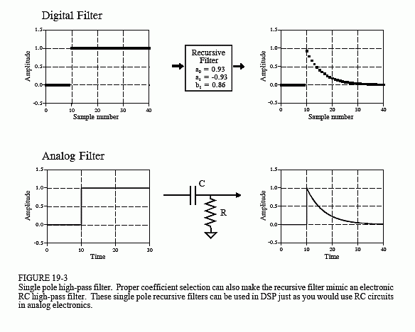
The beauty of the recursive method is in its ability to create a wide variety of responses by changing only a few parameters. For example, Fig. 19-3 shows a filter with three coefficients: a0 = 0.93, a1 = -0.93 and b1 = 0.86. As shown by the similar step responses, this digital filter mimics an electronic RC high-pass filter.
These single pole recursive filters are definitely something you want to keep in your DSP toolbox. You can use them to process digital signals just as you would use RC networks to process analog electronic signals. This includes everything you would expect: DC removal, high-frequency noise suppression, wave shaping, smoothing, etc. They are easy to program, fast

to execute, and produce few surprises. The coefficients are found from these simple equations:


The characteristics of these filters are controlled by the parameter, x, a value between zero and one. Physically, x is the amount of decay between adjacent samples. For instance, x is 0.86 in Fig. 19-3, meaning that the value of each sample in the output signal is 0.86 the value of the sample before it. The higher the value of x, the slower the decay. Notice that the filter becomes unstable if x is made greater than one. That is, any nonzero value on the input will make the output increase until an overflow occurs.

The value for x can be directly specified, or found from the desired time constant of the filter. Just as R×C is the number of seconds it takes an RC circuit to decay to 36.8% of its final value, d is the number of samples it takes for a recursive filter to decay to this same level:

For instance, a sample-to-sample decay of corresponds to a time constant of samples (as shown in Fig 19-3). There is also a fixed relationship between x and the -3dB cutoff frequency, fC, of the digital filter:

This provides three ways to find the "a" and "b" coefficients, starting with the time constant, the cutoff frequency, or just directly picking x.
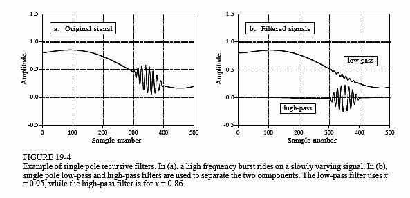
Figure 19-4 shows an example of using single pole recursive filters. In (a), the original signal is a smooth curve, except a burst of a high frequency sine wave. Figure (b) shows the signal after passing through low-pass and high-pass filters. The signals have been separated fairly well, but not perfectly, just as if simple RC circuits were used on an analog signal.

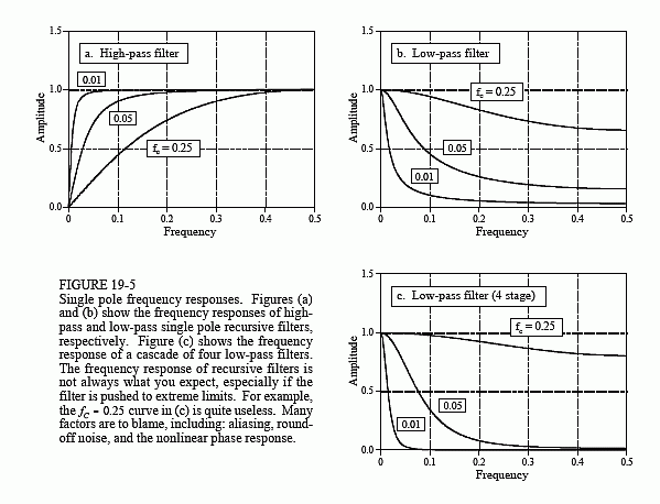
Figure 19-5 shows the frequency responses of various single pole recursive filters. These curves are obtained by passing a delta function through the filter to find the filter's impulse response. The FFT is then used to convert the impulse response into the frequency response. In principle, the impulse response is infinitely long; however, it decays below the single precision round-off noise after about 15 to 20 time constants. For example, when the time constant of the filter is samples, the impulse response can be contained in about 128 samples.
The key feature in Fig. 19-5 is that single pole recursive filters have little ability to separate one band of frequencies from another. In other words, they perform well in the time domain, and poorly in the frequency domain. The frequency response can be improved slightly by cascading several stages. This can be accomplished in two ways. First, the signal can be passed through the filter several times. Second, the z-transform can be used to find the recursion coefficients that combine the cascade into a single stage. Both ways work and are commonly used. Figure (c) shows the frequency response of a cascade of four low-pass filters. Although the stopband attenuation is significantly improved, the roll-off is still terrible. If you need better performance in the frequency domain, look at the Chebyshev filters of the next chapter.
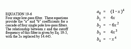
The four stage low-pass filter is comparable to the Blackman and Gaussian filters (relatives of the moving average, Chapter 15), but with a much faster execution speed. The design equations for a four stage low-pass filter are:

