The Scientist and Engineer's Guide to
Digital Signal Processing
By Steven W. Smith, Ph.D.
Book Search

Table of contents
- 1: The Breadth and Depth of DSP
- 2: Statistics, Probability and Noise
- 3: ADC and DAC
- 4: DSP Software
- 5: Linear Systems
- 6: Convolution
- 7: Properties of Convolution
- 8: The Discrete Fourier Transform
- 9: Applications of the DFT
- 10: Fourier Transform Properties
- 11: Fourier Transform Pairs
- 12: The Fast Fourier Transform
- 13: Continuous Signal Processing
- 14: Introduction to Digital Filters
- 15: Moving Average Filters
- 16: Windowed-Sinc Filters
- 17: Custom Filters
- 18: FFT Convolution
- 19: Recursive Filters
- 20: Chebyshev Filters
- 21: Filter Comparison
- 22: Audio Processing
- 23: Image Formation & Display
- 24: Linear Image Processing
- 25: Special Imaging Techniques
- 26: Neural Networks (and more!)
- 27: Data Compression
- 28: Digital Signal Processors
- 29: Getting Started with DSPs
- 30: Complex Numbers
- 31: The Complex Fourier Transform
- 32: The Laplace Transform
- 33: The z-Transform
- 34: Explaining Benford's Law
How to order your own hardcover copy
Wouldn't you rather have a bound book instead of 640 loose pages?Your laser printer will thank you!
Order from Amazon.com.
Chapter 23: Image Formation & Display
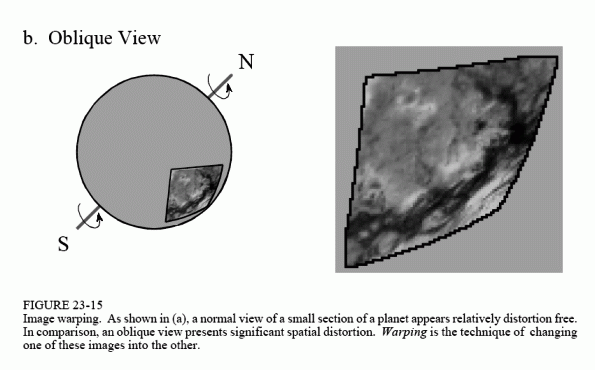
One of the problems in photographing a planet's surface is the distortion from the curvature of the spherical shape. For example, suppose you use a telescope to photograph a square region near the center of a planet, as illustrated in Fig. 23-15a. After a few hours, the planet will have rotated on its axis, appearing as in (b). The previously photographed region appears highly distorted because it is curved near the horizon of the planet. Each of the two images contain complete information about the region, just from a different perspective. It is quite common to acquire a photograph such as (a), but really want the image to look like (b), or vice versa. For example, a satellite mapping the surface of a planet may take thousands of images from straight above, as in (a). To make a natural looking picture of the entire planet, such as the image of Venus in Fig. 23-1, each image must be distorted and placed in the proper position. On the other hand, consider a weather satellite looking at a hurricane that is not directly below it. There is no choice but to acquire the image obliquely, as in (b). The image is then converted into how it would appear from above, as in (a).
These spatial transformations are called warping. Space photography is the most common use for warping, but there are others. For example, many vacuum tube imaging detectors have various amounts of spatial distortion. This includes night vision cameras used by the military and x-ray detectors used in the medical field. Digital warping (or dewarping if you prefer) can be used to correct the inherent distortion in these devices. Special effects artists for motion pictures love to warp images. For example, a technique called morphing gradually warps one object into another over a series of frames. This can produces illusions such as a child turning into an adult, or a man turning into a werewolf.
Warping takes the original image (a two-dimensional array) and generates a warped image (another two-dimensional array). This is done by looping through each pixel in the warped image and asking: What is the proper pixel value that should be placed here? Given the particular row and column being calculated in the warped image, there is a corresponding row and column in the original image. The pixel value from the original image is transferred to the warped image to carry out the algorithm. In the jargon of image processing, the row and column that the pixel comes from in the
original image is called the comes-from address. Transferring each pixel from the original to the warped image is the easy part. The hard part is calculating the comes-from address associated with each pixel in the warped image. This is usually a pure math problem, and can become quite involved. Simply stretching the image in the horizontal or vertical direction is easier, involving only a multiplication of the row and/or column number to find the comes-from address.
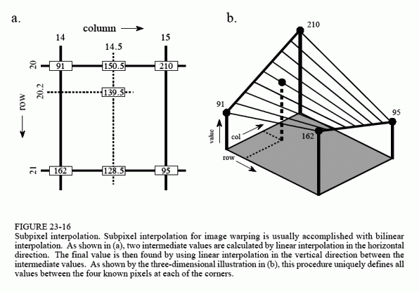
One of the techniques used in warping is subpixel interpolation. For example, suppose you have developed a set of equations that turns a row and column address in the warped image into the comes-from address in the original image. Consider what might happen when you try to find the value of the pixel at row 10 and column 20 in the warped image. You pass the information: row = 10, column = 20, into your equations, and out pops: comes-from row = 20.2, comes-from column = 14.5. The point being, your calculations will likely use floating point, and therefore the comes-from addresses will not be integers. The easiest method to use is the nearest neighbor algorithm, that is, simply round the addresses to the nearest integer. This is simple, but can produce a very grainy appearance at the edges of objects where pixels may appear to be slightly misplaced.
Bilinear interpolation requires a little more effort, but provides significantly better images. Figure 23-16 shows how it works. You know the value of the four pixels around the fractional address, i.e., the value of the pixels at row 20 & 21, and column 14 and 15. In this example we will assume the pixels values are 91, 210, 162 and 95. The problem is to interpolate between these four values. This is done in two steps. First, interpolate in the horizontal direction between column 14 and 15. This produces two intermediate values, 150.5 on line 20, and 128.5 on line 21. Second, interpolate between these intermediate values in the vertical direction. This produces the bilinear interpolated pixel value of 139.5, which is then transferred to the warped image. Why interpolate in the horizontal direction and then the vertical direction instead of the reverse? It doesn't matter; the final answer is the same regardless of which order is used.