The Scientist and Engineer's Guide to
Digital Signal Processing
By Steven W. Smith, Ph.D.
Book Search

Table of contents
- 1: The Breadth and Depth of DSP
- 2: Statistics, Probability and Noise
- 3: ADC and DAC
- 4: DSP Software
- 5: Linear Systems
- 6: Convolution
- 7: Properties of Convolution
- 8: The Discrete Fourier Transform
- 9: Applications of the DFT
- 10: Fourier Transform Properties
- 11: Fourier Transform Pairs
- 12: The Fast Fourier Transform
- 13: Continuous Signal Processing
- 14: Introduction to Digital Filters
- 15: Moving Average Filters
- 16: Windowed-Sinc Filters
- 17: Custom Filters
- 18: FFT Convolution
- 19: Recursive Filters
- 20: Chebyshev Filters
- 21: Filter Comparison
- 22: Audio Processing
- 23: Image Formation & Display
- 24: Linear Image Processing
- 25: Special Imaging Techniques
- 26: Neural Networks (and more!)
- 27: Data Compression
- 28: Digital Signal Processors
- 29: Getting Started with DSPs
- 30: Complex Numbers
- 31: The Complex Fourier Transform
- 32: The Laplace Transform
- 33: The z-Transform
- 34: Explaining Benford's Law
How to order your own hardcover copy
Wouldn't you rather have a bound book instead of 640 loose pages?Your laser printer will thank you!
Order from Amazon.com.
Chapter 34: Explaining Benford's Law
We have looked at two log-normal distributions, one having a standard deviation of 0.25 and the other a standard deviation of 0.5. Surprisingly, one follows Benford's law extremely well, while the other does not follow it at all. In this section we will examine the analytical transition between these two behaviors for this particular distribution.
As shown in Fig. 34-5d, we can use the value of OST(1) as a measure of how well Benford's law is followed. Our goal is to derive an equation relating the standard deviation of psf(g) with the value of OST(1), that is, relating the width of the distribution with its compliance with Benford's law. Notice that this has rigorously defined the problem (removed the fuzziness) by specifying three things, the shape of the distribution, how we are measuring compliance with Benford's law, and how we are defining the distribution width.
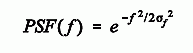
The next step is to write the equation for PSF(f), a one-sided Gaussian curve, having a value of zero at f=0, and a standard deviation of σf:
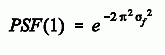
Next we plug in the conversion from the logarithmic-domain standard deviation, σf = 1/(2πσg), and evaluate the expression at f=1:
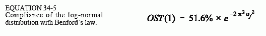
Lastly, we use OST(1) = SF(1) × PSF(1), where SF(1) = 0.516, to reach the final equation:
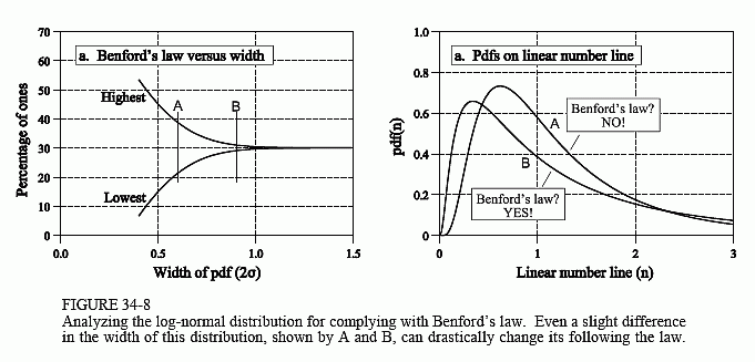
As illustrated in Fig. 34-5c, the highest value in ost(g) is OST(1) plus 0.301, and the lowest value is 0.301 - OST(1). These highest and lowest values are graphed in Fig. 34-8a. As shown, when the 2σ width of the distribution is 0.5 (as in Fig 34-5a), the Ones Scaling Test will have values as high as 45% and as low as 16%, a very poor match to Benford's law. However, doubling the width to 2σ = 1.0 results in a high to low fluctuation of less than 1%, a good match.
There are a number of interesting details in this example. First, notice how rapidly the transition occurs between following and not following Benford's law. For instance, two cases are indicated by A and B in Fig. 34-8, with 2σ = 0.60 and 2σ = 0.90, respectively. In Fig. (b) these are shown on the linear scale. Now imagine that you are a researcher trying to understand Benford's law, before reading this chapter. Even though these two distributions appear very similar, one follows Benford's law very well, and the other doesn't follow it at all! This gives you an idea of the frustration Benford's law has produced.
Second, even though the curves in Fig. (a) move together extremely rapidly, they never actually meet (excluding infinity which isn't allowed for a pdf). For instance, from Eq. 34-5 a log-normal distribution with a standard deviation of three will follow Benford's law within about 1 part in 100,000,000,000,000,000,000,000,000,000,000,000,000,000,000, 000,000,000,000,000,000,000,000,000,000,000. That's pretty close! In fact, you could not statistically detect this error even with a billion computers, each generating a billion numbers each second, since the beginning of the universe.
Nevertheless, this is a finite error, and has caused frustration of its own. Again imagine that you are a researcher trying to understand Benford's law. You proceed by writing down some equation describing when Benford's law will be followed, and then you solve it. The answer you find is– Never! There is no distribution (excluding the oscillatory case of Fig. 34-6b) that follows Benford's law exactly. An equation doesn't give you what is close, only what is equal. In other words, you find no understanding, just more mystery.
Lastly, the log-normal distribution is more than just an example, it is an important case where Benford's law arises in Nature. The reason for this is one of the most powerful driving forces in statistics, the Central Limit Theorem (CLT). As discussed in chapter 2, the CLT describes that adding many random numbers produces a normal distribution. This accounts for the normal distribution being so commonly observed in science and engineering. However, if a group of random numbers are multiplied, the result will be a normal distribution on the logarithmic scale. Accordingly, the log-normal distribution is also commonly found in Nature. This is probably the single most important reason that some distributions are found to follow Benford's law while others do not. Normal distributions are not wide enough to follow the law. On the other hand, broad log-normal distributions follow it to a very high degree.
Want to generate numbers that follow Benford's law for your own experiments? You can take advantage of the CLT. Most computer languages have a random number generator that produces values uniformly distributed between 0 and 1. Call this function multiple times and multiply the numbers. It can be shown that PDF(1) = 0.344 for the uniform distribution, and therefore the product of these numbers follows Benford's law according to OST(1) = 51.6% × 0.344α, where α is how many random numbers are multiplied. For instance, ten multiplications produce a random number that comes from a log-normal distribution with a standard deviation of approximately 0.75. This corresponds to OST(1) = 0.0012%, a very good fit to Benford's law.
If you do try some of these experiments, remember that the statistical variation (noise) on N random events is about SQRT(N). For instance, suppose you generate 1 million numbers in your computer and count how many have 1 as the leading digit. If Benford's law is being followed, this number will be about 301,000. However, when you repeat the experiment several times you find this changes randomly by about 1,000 numbers, since SQRT(1,000,000) = 1,000. In other words, using 1 million numbers allows you to conclude that the percentage of numbers with one as the leading digit is about 30.1% +/- 0.1%. As another example, the ripple in Fig. 34-3a is a result of using 14,414 samples. For a more precise measurement you need more numbers, and it grows very quickly. For instance, to detect the error of OST(1) = 0.0012% (the above example), you will need in excess of a billion numbers.