The Scientist and Engineer's Guide to
Digital Signal Processing
By Steven W. Smith, Ph.D.
Book Search

Table of contents
- 1: The Breadth and Depth of DSP
- 2: Statistics, Probability and Noise
- 3: ADC and DAC
- 4: DSP Software
- 5: Linear Systems
- 6: Convolution
- 7: Properties of Convolution
- 8: The Discrete Fourier Transform
- 9: Applications of the DFT
- 10: Fourier Transform Properties
- 11: Fourier Transform Pairs
- 12: The Fast Fourier Transform
- 13: Continuous Signal Processing
- 14: Introduction to Digital Filters
- 15: Moving Average Filters
- 16: Windowed-Sinc Filters
- 17: Custom Filters
- 18: FFT Convolution
- 19: Recursive Filters
- 20: Chebyshev Filters
- 21: Filter Comparison
- 22: Audio Processing
- 23: Image Formation & Display
- 24: Linear Image Processing
- 25: Special Imaging Techniques
- 26: Neural Networks (and more!)
- 27: Data Compression
- 28: Digital Signal Processors
- 29: Getting Started with DSPs
- 30: Complex Numbers
- 31: The Complex Fourier Transform
- 32: The Laplace Transform
- 33: The z-Transform
- 34: Explaining Benford's Law
How to order your own hardcover copy
Wouldn't you rather have a bound book instead of 640 loose pages?Your laser printer will thank you!
Order from Amazon.com.
Chapter 14: Introduction to Digital Filters
Digital filters are a very important part of DSP. In fact, their extraordinary performance is one of the key reasons that DSP has become so popular. As mentioned in the introduction, filters have two uses: signal separation and signal restoration. Signal separation is needed when a signal has been contaminated with interference, noise, or other signals. For example, imagine a device for measuring the electrical activity of a baby's heart (EKG) while still in the womb. The raw signal will likely be corrupted by the breathing and heartbeat of the mother. A filter might be used to separate these signals so that they can be individually analyzed.
Signal restoration is used when a signal has been distorted in some way. For example, an audio recording made with poor equipment may be filtered to better represent the sound as it actually occurred. Another example is the deblurring of an image acquired with an improperly focused lens, or a shaky camera.
These problems can be attacked with either analog or digital filters. Which is better? Analog filters are cheap, fast, and have a large dynamic range in both amplitude and frequency. Digital filters, in comparison, are vastly superior in the level of performance that can be achieved. For example, a low-pass digital filter presented in Chapter 16 has a gain of 1 +/- 0.0002 from DC to 1000 hertz, and a gain of less than 0.0002 for frequencies above 1001 hertz. The entire transition occurs within only 1 hertz. Don't expect this from an op amp circuit! Digital filters can achieve thousands of times better performance than analog filters. This makes a dramatic difference in how filtering problems are approached. With analog filters, the emphasis is on handling limitations of the electronics, such as the accuracy and stability of the resistors and capacitors. In comparison, digital filters are so good that the performance of the filter is frequently ignored. The emphasis shifts to the limitations of the signals, and the theoretical issues regarding their processing.
It is common in DSP to say that a filter's input and output signals are in the time domain. This is because signals are usually created by sampling at regular intervals of time. But this is not the only way sampling can take place. The second most common way of sampling is at equal intervals in space. For example, imagine taking simultaneous readings from an array of strain sensors mounted at one centimeter increments along the length of an aircraft wing. Many other domains are possible; however, time and space are by far the most common. When you see the term time domain in DSP, remember that it may actually refer to samples taken over time, or it may be a general reference to any domain that the samples are taken in.
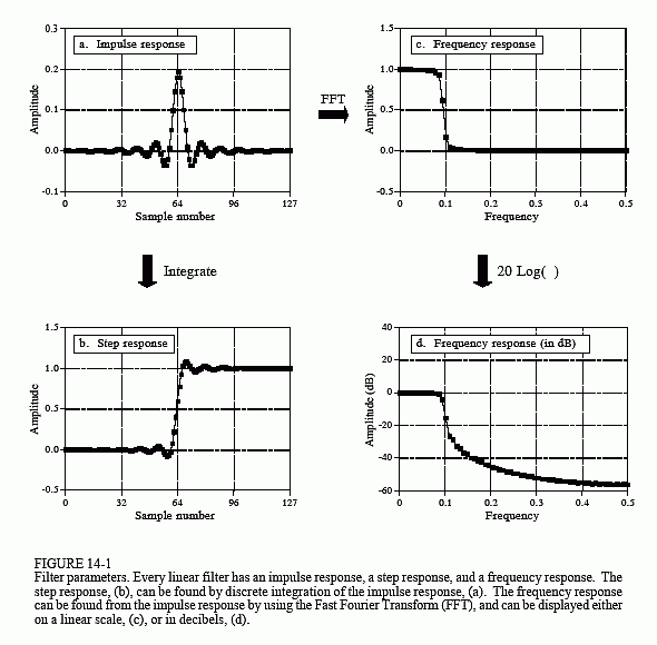
As shown in Fig. 14-1, every linear filter has an impulse response, a step response and a frequency response. Each of these responses contains complete information about the filter, but in a different form. If one of the three is specified, the other two are fixed and can be directly calculated. All three of these representations are important, because they describe how the filter will react under different circumstances.
The most straightforward way to implement a digital filter is by convolving the input signal with the digital filter's impulse response. All possible linear filters can be made in this manner. (This should be obvious. If it isn't, you probably don't have the background to understand this section on filter design. Try reviewing the previous section on DSP fundamentals). When the impulse response is used in this way, filter designers give it a special name: the filter kernel.
There is also another way to make digital filters, called recursion. When a filter is implemented by convolution, each sample in the output is calculated by weighting the samples in the input, and adding them together. Recursive filters are an extension of this, using previously calculated values from the output, besides points from the input. Instead of using a filter kernel, recursive filters are defined by a set of recursion coefficients. This method will be discussed in detail in Chapter 19. For now, the important point is that all linear filters have an impulse response, even if you don't use it to implement the filter. To find the impulse response of a recursive filter, simply feed in an impulse, and see what comes out. The impulse responses of recursive filters are composed of sinusoids that exponentially decay in amplitude. In principle, this makes their impulse responses infinitely long. However, the amplitude eventually drops below the round-off noise of the system, and the remaining samples can be ignored. Because
of this characteristic, recursive filters are also called Infinite Impulse Response or IIR filters. In comparison, filters carried out by convolution are called Finite Impulse Response or FIR filters.
As you know, the impulse response is the output of a system when the input is an impulse. In this same manner, the step response is the output when the input is a step (also called an edge, and an edge response). Since the step is the integral of the impulse, the step response is the integral of the impulse response. This provides two ways to find the step response: (1) feed a step waveform into the filter and see what comes out, or (2) integrate the impulse response. (To be mathematically correct: integration is used with continuous signals, while discrete integration, i.e., a running sum, is used with discrete signals). The frequency response can be found by taking the DFT (using the FFT algorithm) of the impulse response. This will be reviewed later in this chapter. The frequency response can be plotted on a linear vertical axis, such as in (c), or on a logarithmic scale (decibels), as shown in (d). The linear scale is best at showing the passband ripple and roll-off, while the decibel scale is needed to show the stopband attenuation.
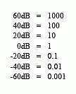
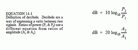
Don't remember decibels? Here is a quick review. A bel (in honor of Alexander Graham Bell) means that the power is changed by a factor of ten. For example, an electronic circuit that has 3 bels of amplification produces an output signal with 10 × 10 × 10 = 1000 times the power of the input. A decibel (dB) is one-tenth of a bel. Therefore, the decibel values of: -20dB, -10dB, 0dB, 10dB & 20dB, mean the power ratios: 0.01, 0.1, 1, 10, & 100, respectively. In other words, every ten decibels mean that the power has changed by a factor of ten.
Here's the catch: you usually want to work with a signal's amplitude, not its power. For example, imagine an amplifier with 20dB of gain. By definition, this means that the power in the signal has increased by a factor of 100. Since amplitude is proportional to the square-root of power, the amplitude of the output is 10 times the amplitude of the input. While 20dB means a factor of 100 in power, it only means a factor of 10 in amplitude. Every twenty decibels mean that the amplitude has changed by a factor of ten. In equation form:
The above equations use the base 10 logarithm; however, many computer languages only provide a function for the base e logarithm (the natural log, written logex or ln x ). The natural log can be use by modifying the above equations: dB = 4.342945 loge(P2/P1) and dB = 8.685890 loge(A2/A1).
Since decibels are a way of expressing the ratio between two signals, they are ideal for describing the gain of a system, i.e., the ratio between the output and the input signal. However, engineers also use decibels to specify the amplitude (or power) of a single signal, by referencing it to some standard. For example, the term: dBV means that the signal is being referenced to a 1 volt rms signal. Likewise, dBm indicates a reference signal producing 1 mW into a 600 ohms load (about 0.78 volts rms).
If you understand nothing else about decibels, remember two things: First, -3dB means that the amplitude is reduced to 0.707 (and the power is therefore reduced to 0.5). Second, memorize the following conversions between decibels and amplitude ratios: