The Scientist and Engineer's Guide to
Digital Signal Processing
By Steven W. Smith, Ph.D.
Book Search

Table of contents
- 1: The Breadth and Depth of DSP
- 2: Statistics, Probability and Noise
- 3: ADC and DAC
- 4: DSP Software
- 5: Linear Systems
- 6: Convolution
- 7: Properties of Convolution
- 8: The Discrete Fourier Transform
- 9: Applications of the DFT
- 10: Fourier Transform Properties
- 11: Fourier Transform Pairs
- 12: The Fast Fourier Transform
- 13: Continuous Signal Processing
- 14: Introduction to Digital Filters
- 15: Moving Average Filters
- 16: Windowed-Sinc Filters
- 17: Custom Filters
- 18: FFT Convolution
- 19: Recursive Filters
- 20: Chebyshev Filters
- 21: Filter Comparison
- 22: Audio Processing
- 23: Image Formation & Display
- 24: Linear Image Processing
- 25: Special Imaging Techniques
- 26: Neural Networks (and more!)
- 27: Data Compression
- 28: Digital Signal Processors
- 29: Getting Started with DSPs
- 30: Complex Numbers
- 31: The Complex Fourier Transform
- 32: The Laplace Transform
- 33: The z-Transform
- 34: Explaining Benford's Law
How to order your own hardcover copy
Wouldn't you rather have a bound book instead of 640 loose pages?Your laser printer will thank you!
Order from Amazon.com.
Chapter 26: Neural Networks (and more!)
Scientists & engineers often need to know if a particular object or condition is present. For instance, geophysicists explore the earth for oil, physicians examine patients for disease, astronomers search the universe for extra-terrestrial intelligence, etc. These problems usually involve comparing the acquired data against a threshold. If the threshold is exceeded, the target (the object or condition being sought) is deemed present.
For example, suppose you invent a device for detecting cancer in humans. The apparatus is waved over a patient, and a number between 0 and 30 pops up on the video screen. Low numbers correspond to healthy subjects, while high numbers indicate that cancerous tissue is present. You find that the device works quite well, but isn't perfect and occasionally makes an error. The question is: how do you use this system to the benefit of the patient being examined?
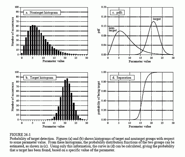
Figure 26-1 illustrates a systematic way of analyzing this situation. Suppose the device is tested on two groups: several hundred volunteers known to be healthy (nontarget), and several hundred volunteers known to have cancer (target). Figures (a) & (b) show these test results displayed as histograms. The healthy subjects generally produce a lower number than those that have cancer (good), but there is some overlap between the two distributions (bad).
As discussed in Chapter 2, the histogram can be used as an estimate of the probability distribution function (pdf), as shown in (c). For instance, imagine that the device is used on a randomly chosen healthy subject. From (c), there is about an 8% chance that the test result will be 3, about a 1% chance that it will be 18, etc. (This example does not specify if the output is a real number, requiring a pdf, or an integer, requiring a pmf. Don't worry about it here; it isn't important).
Now, think about what happens when the device is used on a patient of unknown health. For example, if a person we have never seen before receives a value of 15, what can we conclude? Do they have cancer or not? We know that the probability of a healthy person generating a 15 is 2.1%. Likewise, there is a 0.7% chance that a person with cancer will produce a 15. If no other information is available, we would conclude that the subject is three times as likely not to have cancer, as to have cancer. That is, the test result of 15 implies a 25% probability that the subject is from the target group. This method can be generalized to form the curve in (d), the probability of the subject having cancer based only on the number produced by the device [mathematically, pdft/(pdft + pdfnt)].
If we stopped the analysis at this point, we would be making one of the most common (and serious) errors in target detection. Another source of information must usually be taken into account to make the curve in (d) meaningful. This is the relative number of targets versus nontargets in the population to be tested. For instance, we may find that only one in one-thousand people have the cancer we are trying to detect. To include this in the analysis, the amplitude of the nontarget pdf in (c) is adjusted so that the area under the curve is 0.999. Likewise, the amplitude of the target pdf is adjusted to make the area under the curve be 0.001. Figure (d) is then calculated as before to give the probability that a patient has cancer.
Neglecting this information is a serious error because it greatly affects how the test results are interpreted. In other words, the curve in figure (d) is drastically altered when the prevalence information is included. For instance, if the fraction of the population having cancer is 0.001, a test result of 15 corresponds to only a 0.025% probability that this patient has cancer. This is very different from the 25% probability found by relying on the output of the machine alone.
This method of converting the output value into a probability can be useful for understanding the problem, but it is not the main way that target detection is accomplished. Most applications require a yes/no decision on
the presence of a target, since yes will result in one action and no will result in another. This is done by comparing the output value of the test to a threshold. If the output is above the threshold, the test is said to be positive, indicating that the target is present. If the output is below the threshold, the test is said to be negative, indicating that the target is not present. In our cancer example, a negative test result means that the patient is told they are healthy, and sent home. When the test result is positive, additional tests will be performed, such as obtaining a sample of the tissue by insertion of a biopsy needle.
Since the target and nontarget distributions overlap, some test results will not be correct. That is, some patients sent home will actually have cancer, and some patients sent for additional tests will be healthy. In the jargon of target detection, a correct classification is called true, while an incorrect classification is called false. For example, if a patient has cancer, and the test properly detects the condition, it is said to be a true-positive. Likewise, if a patient does not have cancer, and the test indicates that cancer is not present, it is said to be a true-negative. A false-positive occurs when the patient does not have cancer, but the test erroneously indicates that they do. This results in needless worry, and the pain and expense of additional tests. An even worse scenario occurs with the false-negative, where cancer is present, but the test indicates the patient is healthy. As we all know, untreated cancer can cause many health problems, including premature death.
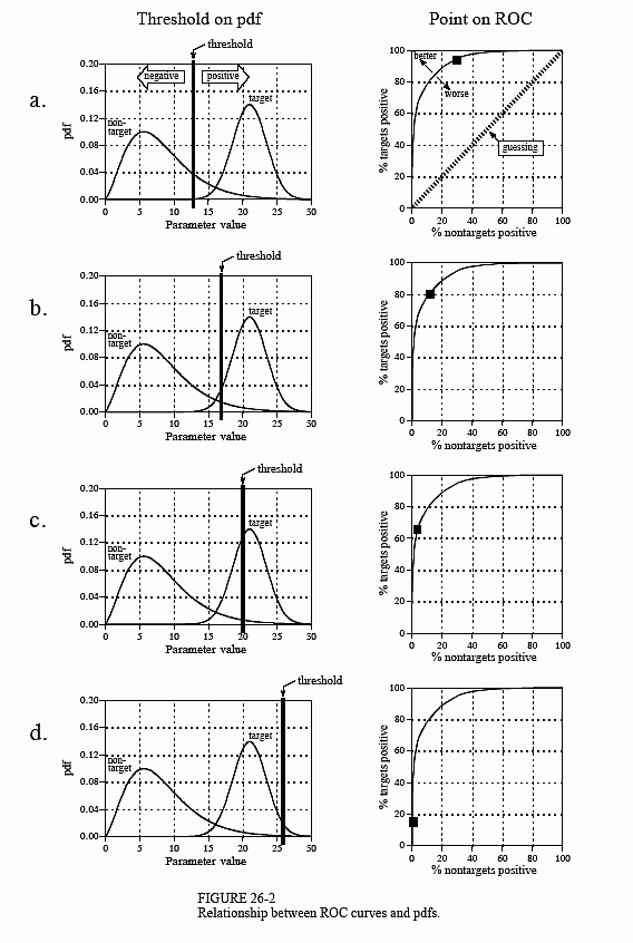
The human suffering resulting from these two types of errors makes the threshold selection a delicate balancing act. How many false-positives can be tolerated to reduce the number of false-negatives? Figure 26-2 shows a graphical way of evaluating this problem, the ROC curve (short for Receiver Operating Characteristic). The ROC curve plots the percent of target signals reported as positive (higher is better), against the percent of nontarget signals erroneously reported as positive (lower is better), for various values of the threshold. In other words, each point on the ROC curve represents one possible tradeoff of true-positive and false-positive performance.
Figures (a) through (d) show four settings of the threshold in our cancer detection example. For instance, look at (b) where the threshold is set at 17. Remember, every test that produces an output value greater than the threshold is reported as a positive result. About 13% of the area of the nontarget distribution is greater than the threshold (i.e., to the right of the threshold). Of all the patients that do not have cancer, 87% will be reported as negative (i.e., a true-negative), while 13% will be reported as positive (i.e., a false-positive). In comparison, about 80% of the area of the target distribution is greater than the threshold. This means that 80% of those that have cancer will generate a positive test result (i.e., a true-positive). The other 20% that have cancer will be incorrectly reported as a negative (i.e., a false-negative). As shown in the ROC curve in (b), this threshold results in a point on the curve at: % nontargets positive = 13%, and % targets positive = 80%.
The more efficient the detection process, the more the ROC curve will bend toward the upper-left corner of the graph. Pure guessing results in a straight line at a 45° diagonal. Setting the threshold relatively low, as shown in (a), results in nearly all the target signals being detected. This comes at the price of many false alarms (false-positives). As illustrated in (d), setting the threshold relatively high provides the reverse situation: few false alarms, but many missed targets.
These analysis techniques are useful in understanding the consequences of threshold selection, but the final decision is based on what some human will accept. Suppose you initially set the threshold of the cancer detection apparatus to some value you feel is appropriate. After many patients have been screened with the system, you speak with a dozen or so patients that have been subjected to false-positives. Hearing how your system has unnecessarily disrupted the lives of these people affects you deeply, motivating you to increase the threshold. Eventually you encounter a
situation that makes you feel even worse: you speak with a patient who is terminally ill with a cancer that your system failed to detect. You respond to this difficult experience by greatly lowering the threshold. As time goes on and these events are repeated many times, the threshold gradually moves to an equilibrium value. That is, the false-positive rate multiplied by a significance factor (lowering the threshold) is balanced by the false-negative rate multiplied by another significance factor (raising the threshold).
This analysis can be extended to devices that provide more than one output. For example, suppose that a cancer detection system operates by taking an x-ray image of the subject, followed by automated image analysis algorithms to identify tumors. The algorithms identify suspicious regions, and then measure key characteristics to aid in the evaluation. For instance, suppose we measure the diameter of the suspect region (parameter 1) and its brightness in the image (parameter 2). Further suppose that our research indicates that tumors are generally larger and brighter than normal tissue. As a first try, we could go through the previously presented ROC analysis for each parameter, and find an acceptable threshold for each. We could then classify a test as positive only if it met both criteria: parameter 1 greater than some threshold and parameter 2 greater than another threshold.
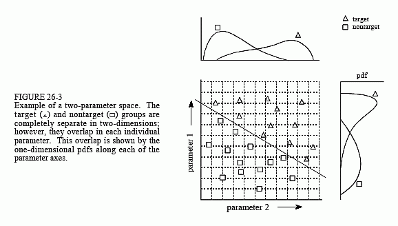
This technique of thresholding the parameters separately and then invoking logic functions (AND, OR, etc.) is very common. Nevertheless, it is very inefficient, and much better methods are available. Figure 26-3 shows why this is the case. In this figure, each triangle represents a single occurrence of a target (a patient with cancer), plotted at a location that corresponds to the value of its two parameters. Likewise, each square represents a single occurrence of a nontarget (a patient without cancer). As shown in the pdf
graph on the side of each axis, both parameters have a large overlap between the target and nontarget distributions. In other words, each parameter, taken individually, is a poor predictor of cancer. Combining the two parameters with simple logic functions would only provide a small improvement. This is especially interesting since the two parameters contain information to perfectly separate the targets from the nontargets. This is done by drawing a diagonal line between the two groups, as shown in the figure.
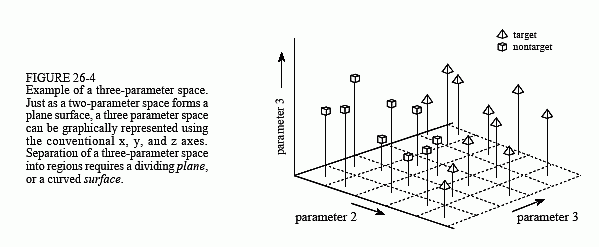
In the jargon of the field, this type of coordinate system is called a parameter space. For example, the two-dimensional plane in this example could be called a diameter-brightness space. The idea is that targets will occupy one region of the parameter space, while nontargets will occupy another. Separation between the two regions may be as simple as a straight line, or as complicated as closed regions with irregular borders. Figure 26-4 shows the next level of complexity, a three-parameter space being represented on the x, y and z axes. For example, this might correspond to a cancer detection system that measures diameter, brightness, and some third parameter, say, edge sharpness. Just as in the two-dimensional case, the important idea is that the members of the target and nontarget groups will (hopefully) occupy different regions of the space, allowing the two to be separated. In three dimensions, regions are separated by planes and curved surfaces. The term hyperspace (over, above, or beyond normal space) is often used to describe parameter spaces with more than three dimensions. Mathematically, hyperspaces are no different from one, two and three-dimensional spaces; however, they have the practical problem of not being able to be displayed in a graphical form in our three-dimensional universe.
The threshold selected for a single parameter problem cannot (usually) be classified as right or wrong. This is because each threshold value results in a unique combination of false-positives and false-negatives, i.e., some point along the ROC curve. This is trading one goal for another, and has no absolutely correct answer. On the other hand, parameter spaces with two or more parameters can definitely have wrong divisions between regions. For instance, imagine increasing the number of data points in Fig. 26-3, revealing a small overlap between the target and nontarget groups. It would be possible to move the threshold line between the groups to trade the number of false-positives against the number of false-negatives. That is, the diagonal line would be moved toward the top-right, or the bottom-left. However, it would be wrong to rotate the line, because it would increase both types of errors.
As suggested by these examples, the conventional approach to target detection (sometimes called pattern recognition) is a two step process. The first step is called feature extraction. This uses algorithms to reduce the raw data to a few parameters, such as diameter, brightness, edge sharpness, etc. These parameters are often called features or classifiers. Feature extraction is needed to reduce the amount of data. For example, a medical x-ray image may contain more than a million pixels. The goal of feature extraction is to distill the information into a more concentrated and manageable form. This type of algorithm development is more of an art than a science. It takes a great deal of experience and skill to look at a problem and say: "These are the classifiers that best capture the information." Trial-and-error plays a significant role.
In the second step, an evaluation is made of the classifiers to determine if the target is present or not. In other words, some method is used to divide the parameter space into a region that corresponds to the targets, and a region that corresponds to the nontargets. This is quite straightforward for one and two-parameter spaces; the known data points are plotted on a graph (such as Fig. 26-3), and the regions separated by eye. The division is then written into a computer program as an equation, or some other way of defining one region from another. In principle, this same technique can be applied to a three-dimensional parameter space. The problem is, three-dimensional graphs are very difficult for humans to understand and visualize (such as Fig. 26-4). Caution: Don't try this in hyperspace; your brain will explode!
In short, we need a machine that can carry out a multi-parameter space division, according to examples of target and nontarget signals. This ideal target detection system is remarkably close to the main topic of this chapter, the neural network.