The Scientist and Engineer's Guide to
Digital Signal Processing
By Steven W. Smith, Ph.D.
Book Search

Table of contents
- 1: The Breadth and Depth of DSP
- 2: Statistics, Probability and Noise
- 3: ADC and DAC
- 4: DSP Software
- 5: Linear Systems
- 6: Convolution
- 7: Properties of Convolution
- 8: The Discrete Fourier Transform
- 9: Applications of the DFT
- 10: Fourier Transform Properties
- 11: Fourier Transform Pairs
- 12: The Fast Fourier Transform
- 13: Continuous Signal Processing
- 14: Introduction to Digital Filters
- 15: Moving Average Filters
- 16: Windowed-Sinc Filters
- 17: Custom Filters
- 18: FFT Convolution
- 19: Recursive Filters
- 20: Chebyshev Filters
- 21: Filter Comparison
- 22: Audio Processing
- 23: Image Formation & Display
- 24: Linear Image Processing
- 25: Special Imaging Techniques
- 26: Neural Networks (and more!)
- 27: Data Compression
- 28: Digital Signal Processors
- 29: Getting Started with DSPs
- 30: Complex Numbers
- 31: The Complex Fourier Transform
- 32: The Laplace Transform
- 33: The z-Transform
- 34: Explaining Benford's Law
How to order your own hardcover copy
Wouldn't you rather have a bound book instead of 640 loose pages?Your laser printer will thank you!
Order from Amazon.com.
Chapter 12: The Fast Fourier Transform
J.W. Cooley and J.W. Tukey are given credit for bringing the FFT to the world in their paper: "An algorithm for the machine calculation of complex Fourier Series," Mathematics Computation, Vol. 19, 1965, pp 297-301. In retrospect, others had discovered the technique many years before. For instance, the great German mathematician Karl Friedrich Gauss (1777-1855) had used the method more than a century earlier. This early work was largely forgotten because it lacked the tool to make it practical: the digital computer. Cooley and Tukey are honored because they discovered the FFT at the right time, the beginning of the computer revolution.
The FFT is based on the complex DFT, a more sophisticated version of the real DFT discussed in the last four chapters. These transforms are named for the way each represents data, that is, using complex numbers or using real numbers. The term complex does not mean that this representation is difficult or complicated, but that a specific type of mathematics is used. Complex mathematics often is difficult and complicated, but that isn't where the name comes from. Chapter 29 discusses the complex DFT and provides the background needed to understand the details of the FFT algorithm. The
topic of this chapter is simpler: how to use the FFT to calculate the real DFT, without drowning in a mire of advanced mathematics.
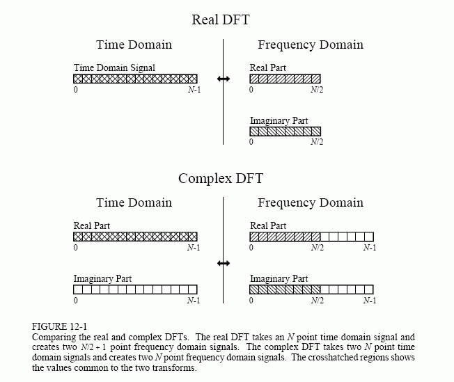
Since the FFT is an algorithm for calculating the complex DFT, it is important to understand how to transfer real DFT data into and out of the complex DFT format. Figure 12-1 compares how the real DFT and the complex DFT store data. The real DFT transforms an N point time domain signal into two N/2 + 1 point frequency domain signals. The time domain signal is called just that: the time domain signal. The two signals in the frequency domain are called the real part and the imaginary part, holding the amplitudes of the cosine waves and sine waves, respectively. This should be very familiar from past chapters.
In comparison, the complex DFT transforms two N point time domain signals into two N point frequency domain signals. The two time domain signals are called the real part and the imaginary part, just as are the frequency domain signals. In spite of their names, all of the values in these arrays are just ordinary numbers. (If you are familiar with complex numbers: the j's are not included in the array values; they are a part of the mathematics. Recall that the operator, Im( ), returns a real number).
Suppose you have an N point signal, and need to calculate the real DFT by means of the Complex DFT (such as by using the FFT algorithm). First, move the N point signal into the real part of the complex DFT's time domain, and then set all of the samples in the imaginary part to zero. Calculation of the complex DFT results in a real and an imaginary signal in the frequency domain, each composed of N points. Samples 0 through N/2 of these signals correspond to the real DFT's spectrum.
As discussed in Chapter 10, the DFT's frequency domain is periodic when the negative frequencies are included (see Fig. 10-9). The choice of a single period is arbitrary; it can be chosen between -1.0 and 0, -0.5 and 0.5, 0 and 1.0, or any other one unit interval referenced to the sampling rate. The complex DFT's frequency spectrum includes the negative frequencies in the 0 to 1.0 arrangement. In other words, one full period stretches from sample 0 to sample N-1, corresponding with 0 to 1.0 times the sampling rate. The positive frequencies sit between sample 0 and N/2, corresponding with 0 to 0.5. The other samples, between N/2 + 1 and N - 1, contain the negative frequency values (which are usually ignored).
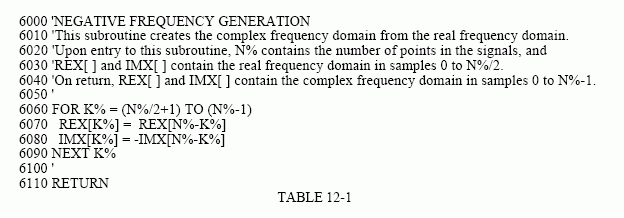
Calculating a real Inverse DFT using a complex Inverse DFT is slightly harder. This is because you need to insure that the negative frequencies are loaded in the proper format. Remember, points 0 through N/2 in the complex DFT are the same as in the real DFT, for both the real and the imaginary parts. For the real part, point N/2 + 1 is the same as point N/2 - 1, point N/2 + 2 is the same as point N/2 - 2, etc. This continues to point N-1 being the same as point 1. The same basic pattern is used for the imaginary part, except the sign is changed. That is, point N/2 + 1 is the negative of point N/2 - 1, point N/2 + 2 is the negative of point N/2 - 2, etc. Notice that samples 0 and N/2 do not have a matching point in this duplication scheme. Use Fig. 10-9 as a guide to understanding this symmetry. In practice, you load the real DFT's frequency spectrum into samples 0 to N/2 of the complex DFT's arrays, and then use a subroutine to generate the negative frequencies between samples N/2 + 1 and N-1 . Table 12-1 shows such a program. To check that the proper symmetry is present, after taking the inverse FFT, look at the imaginary part of the time domain. It will contain all zeros if everything is correct (except for a few parts-per-million of noise, using single precision calculations).