The Scientist and Engineer's Guide to
Digital Signal Processing
By Steven W. Smith, Ph.D.
Book Search

Table of contents
- 1: The Breadth and Depth of DSP
- 2: Statistics, Probability and Noise
- 3: ADC and DAC
- 4: DSP Software
- 5: Linear Systems
- 6: Convolution
- 7: Properties of Convolution
- 8: The Discrete Fourier Transform
- 9: Applications of the DFT
- 10: Fourier Transform Properties
- 11: Fourier Transform Pairs
- 12: The Fast Fourier Transform
- 13: Continuous Signal Processing
- 14: Introduction to Digital Filters
- 15: Moving Average Filters
- 16: Windowed-Sinc Filters
- 17: Custom Filters
- 18: FFT Convolution
- 19: Recursive Filters
- 20: Chebyshev Filters
- 21: Filter Comparison
- 22: Audio Processing
- 23: Image Formation & Display
- 24: Linear Image Processing
- 25: Special Imaging Techniques
- 26: Neural Networks (and more!)
- 27: Data Compression
- 28: Digital Signal Processors
- 29: Getting Started with DSPs
- 30: Complex Numbers
- 31: The Complex Fourier Transform
- 32: The Laplace Transform
- 33: The z-Transform
- 34: Explaining Benford's Law
How to order your own hardcover copy
Wouldn't you rather have a bound book instead of 640 loose pages?Your laser printer will thank you!
Order from Amazon.com.
Chapter 15: Moving Average Filters
In a perfect world, filter designers would only have to deal with time domain or frequency domain encoded information, but never a mixture of the two in the same signal. Unfortunately, there are some applications where both domains are simultaneously important. For instance, television signals fall into this nasty category. Video information is encoded in the time domain, that is, the shape of the waveform corresponds to the patterns of brightness in the image. However, during transmission the video signal is treated according to its frequency composition, such as its total bandwidth, how the carrier waves for sound & color are added, elimination & restoration of the DC component, etc. As another example, electro-magnetic interference is best understood in the frequency domain, even if
the signal's information is encoded in the time domain. For instance, the temperature monitor in a scientific experiment might be contaminated with 60 hertz from the power lines, 30 kHz from a switching power supply, or 1320 kHz from a local AM radio station. Relatives of the moving average filter have better frequency domain performance, and can be useful in these mixed domain applications.
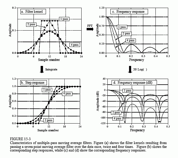
Multiple-pass moving average filters involve passing the input signal through a moving average filter two or more times. Figure 15-3a shows the overall filter kernel resulting from one, two and four passes. Two passes are equivalent to using a triangular filter kernel (a rectangular filter kernel convolved with itself). After four or more passes, the equivalent filter kernel looks like a Gaussian (recall the Central Limit Theorem). As shown in (b), multiple passes produce an "s" shaped step response, as compared to the straight line of the single pass. The frequency responses in (c) and (d) are given by Eq. 15-2 multiplied by itself for each pass. That is, each time domain convolution results in a multiplication of the frequency spectra.
Figure 15-4 shows the frequency response of two other relatives of the moving average filter. When a pure Gaussian is used as a filter kernel, the frequency response is also a Gaussian, as discussed in Chapter 11. The Gaussian is important because it is the impulse response of many natural and manmade systems. For example, a brief pulse of light entering a long fiber optic transmission line will exit as a Gaussian pulse, due to the different paths taken by the photons within the fiber. The Gaussian filter kernel is also used extensively in image processing because it has unique properties that allow fast two-dimensional convolutions (see Chapter 24). The second frequency response in Fig. 15-4 corresponds to using a Blackman window as a filter kernel. (The term window has no meaning here; it is simply part of the accepted name of this curve). The exact shape of the Blackman window is given in Chapter 16 (Eq. 16-2, Fig. 16-2); however, it looks much like a Gaussian.
How are these relatives of the moving average filter better than the moving average filter itself? Three ways: First, and most important, these filters have better stopband attenuation than the moving average filter. Second, the filter kernels taper to a smaller amplitude near the ends. Recall that each point in the output signal is a weighted sum of a group of samples from the input. If the filter kernel tapers, samples in the input signal that are farther away are given less weight than those close by. Third, the step responses are smooth curves, rather than the abrupt straight line of the moving average. These last two are usually of limited benefit, although you might find applications where they are genuine advantages.
The moving average filter and its relatives are all about the same at reducing random noise while maintaining a sharp step response. The ambiguity lies in how the risetime of the step response is measured. If the risetime is measured from 0% to 100% of the step, the moving average filter is the best you can do, as previously shown. In comparison, measuring the risetime from 10% to 90% makes the Blackman window better than the moving average filter. The point is, this is just theoretical squabbling; consider these filters equal in this parameter.
The biggest difference in these filters is execution speed. Using a recursive algorithm (described next), the moving average filter will run like lightning in your computer. In fact, it is the fastest digital filter available. Multiple passes of the moving average will be correspondingly slower, but still very quick. In comparison, the Gaussian and Blackman filters are excruciatingly slow, because they must use convolution. Think a factor of ten times the number of points in the filter kernel (based on multiplication being about 10 times slower than addition). For example, expect a 100 point Gaussian to be 1000 times slower than a moving average using recursion.