The Scientist and Engineer's Guide to
Digital Signal Processing
By Steven W. Smith, Ph.D.
Book Search
Table of contents
- 1: The Breadth and Depth of DSP
- 2: Statistics, Probability and Noise
- 3: ADC and DAC
- 4: DSP Software
- 5: Linear Systems
- 6: Convolution
- 7: Properties of Convolution
- 8: The Discrete Fourier Transform
- 9: Applications of the DFT
- 10: Fourier Transform Properties
- 11: Fourier Transform Pairs
- 12: The Fast Fourier Transform
- 13: Continuous Signal Processing
- 14: Introduction to Digital Filters
- 15: Moving Average Filters
- 16: Windowed-Sinc Filters
- 17: Custom Filters
- 18: FFT Convolution
- 19: Recursive Filters
- 20: Chebyshev Filters
- 21: Filter Comparison
- 22: Audio Processing
- 23: Image Formation & Display
- 24: Linear Image Processing
- 25: Special Imaging Techniques
- 26: Neural Networks (and more!)
- 27: Data Compression
- 28: Digital Signal Processors
- 29: Getting Started with DSPs
- 30: Complex Numbers
- 31: The Complex Fourier Transform
- 32: The Laplace Transform
- 33: The z-Transform
- 34: Explaining Benford's Law
How to order your own hardcover copy
Wouldn't you rather have a bound book instead of 640 loose pages?Your laser printer will thank you!
Order from Amazon.com.
Chapter 8: The Discrete Fourier Transform
Pulling together everything said so far, we can write the synthesis equation:

In words, any N point signal, x[i], can be created by adding N/2 + 1 cosine waves and N/2 + 1 sine waves. The amplitudes of the cosine and sine waves are held in the arrays ImX[k] and ReX[k], respectively. The synthesis equation multiplies these amplitudes by the basis functions to create a set of scaled sine and cosine waves. Adding the scaled sine and cosine waves produces the time domain signal, x[i].
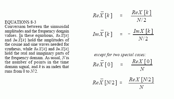
In Eq. 8-2, the arrays are called ImX[k] and ReX[k], rather than ImX[k] and ReX[k]. This is because the amplitudes needed for synthesis (called in this discussion: ImX[k] and ReX[k]), are slightly different from the frequency domain of a signal (denoted by: ImX[k] and ReX[k]). This is the scaling factor issue we referred to earlier. Although the conversion is only a simple normalization, it is a common bug in computer programs. Look out for it! In equation form, the conversion between the two is given by:

Suppose you are given a frequency domain representation, and asked to synthesize the corresponding time domain signal. To start, you must find the amplitudes of the sine and cosine waves. In other words, given ImX[k] and ReX[k], you must find ImX[k] and ReX[k]. Equation 8-3 shows this in a mathematical form. To do this in a computer program, three actions must be taken. First, divide all the values in the frequency domain by N/2. Second, change the sign of all the imaginary values. Third, divide the first and last samples in the real part, ReX[0] and ReX[N/2], by two. This provides the amplitudes needed for the synthesis described by Eq. 8-2. Taken together, Eqs. 8-2 and 8-3 define the inverse DFT.
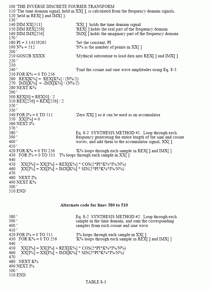
The entire Inverse DFT is shown in the computer program listed in Table 8-1. There are two ways that the synthesis (Eq. 8-2) can be programmed, and both are shown. In the first method, each of the scaled sinusoids are generated one at a time and added to an accumulation array, which ends up becoming the time domain signal. In the second method, each sample in the time domain signal is calculated one at a time, as the sum of all the


corresponding samples in the cosine and sine waves. Both methods produce the same result. The difference between these two programs is very minor; the inner and outer loops are swapped during the synthesis.
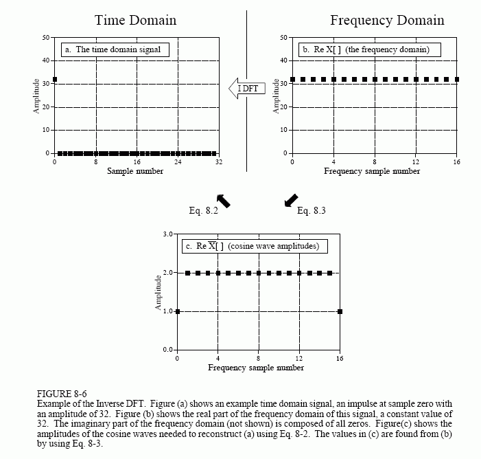
Figure 8-6 illustrates the operation of the Inverse DFT, and the slight differences between the frequency domain and the amplitudes needed for synthesis. Figure 8-6a is an example signal we wish to synthesize, an impulse at sample zero with an amplitude of 32. Figure 8-6b shows the frequency domain representation of this signal. The real part of the frequency domain is a constant value of 32. The imaginary part (not shown) is composed of all zeros. As discussed in the next chapter, this is an important DFT pair: an impulse in the time domain corresponds to a constant value in the frequency domain. For now, the important point is that (b) is the DFT of (a), and (a) is the Inverse DFT of (b).
Equation 8-3 is used to convert the frequency domain signal, (b), into the amplitudes of the cosine waves, (c). As shown, all of the cosine waves have an amplitude of two, except for samples 0 and 16, which have a value of one. The amplitudes of the sine waves are not shown in this example because they have a value of zero, and therefore provide no contribution. The synthesis equation, Eq. 8-2, is then used to convert the amplitudes of the cosine waves, (b), into the time domain signal, (a).
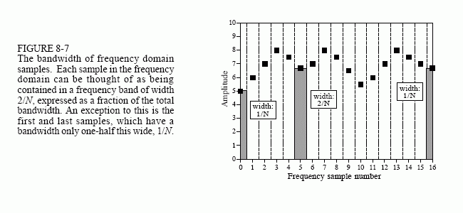
This describes how the frequency domain is different from the sinusoidal amplitudes, but it doesn't explain why it is different. The difference occurs because the frequency domain is defined as a spectral density. Figure 8-7 shows how this works. The example in this figure is the real part of the frequency domain of a 32 point signal. As you should expect, the samples run from 0 to 16, representing 17 frequencies equally spaced between 0 and 1/2 of the sampling rate. Spectral density describes how much signal (amplitude) is present per unit of bandwidth. To convert the sinusoidal amplitudes into a spectral density, divide each amplitude by the bandwidth represented by each amplitude. This brings up the next issue: how do we determine the bandwidth of each of the discrete frequencies in the frequency domain?
As shown in the figure, the bandwidth can be defined by drawing dividing lines between the samples. For instance, sample number 5 occurs in the band between 4.5 and 5.5; sample number 6 occurs in the band between 5.5 and 6.5, etc. Expressed as a fraction of the total bandwidth (i.e., ), the bandwidth of each sample is 2/N. An exception to this is the samples on each end, which have one-half of this bandwidth, . This accounts for the scaling factor between the sinusoidal amplitudes and frequency domain, as well as the additional factor of two needed for the first and last samples.
Why the negation of the imaginary part? This is done solely to make the real DFT consistent with its big brother, the complex DFT. In Chapter 29 we will show that it is necessary to make the mathematics of the complex DFT work. When dealing only with the real DFT, many authors do not include this negation. For that matter, many authors do not even include

the 2/N scaling factor. Be prepared to find both of these missing in some discussions. They are included here for a tremendously important reason: The most efficient way to calculate the DFT is through the Fast Fourier Transform (FFT) algorithm, presented in Chapter 12. The FFT generates a frequency domain defined according to Eq. 8-2 and 8-3. If you start messing with these normalization factors, your programs containing the FFT are not going to work as expected.
