The Scientist and Engineer's Guide to
Digital Signal Processing
By Steven W. Smith, Ph.D.
Book Search

Table of contents
- 1: The Breadth and Depth of DSP
- 2: Statistics, Probability and Noise
- 3: ADC and DAC
- 4: DSP Software
- 5: Linear Systems
- 6: Convolution
- 7: Properties of Convolution
- 8: The Discrete Fourier Transform
- 9: Applications of the DFT
- 10: Fourier Transform Properties
- 11: Fourier Transform Pairs
- 12: The Fast Fourier Transform
- 13: Continuous Signal Processing
- 14: Introduction to Digital Filters
- 15: Moving Average Filters
- 16: Windowed-Sinc Filters
- 17: Custom Filters
- 18: FFT Convolution
- 19: Recursive Filters
- 20: Chebyshev Filters
- 21: Filter Comparison
- 22: Audio Processing
- 23: Image Formation & Display
- 24: Linear Image Processing
- 25: Special Imaging Techniques
- 26: Neural Networks (and more!)
- 27: Data Compression
- 28: Digital Signal Processors
- 29: Getting Started with DSPs
- 30: Complex Numbers
- 31: The Complex Fourier Transform
- 32: The Laplace Transform
- 33: The z-Transform
- 34: Explaining Benford's Law
How to order your own hardcover copy
Wouldn't you rather have a bound book instead of 640 loose pages?Your laser printer will thank you!
Order from Amazon.com.
Chapter 13: Continuous Signal Processing
The Fourier Transform for continuous signals is divided into two categories, one for signals that are periodic, and one for signals that are aperiodic. Periodic signals use a version of the Fourier Transform called the Fourier Series, and are discussed in the next section. The Fourier Transform used with aperiodic signals is simply called the Fourier Transform. This chapter describes these Fourier techniques using only real mathematics, just as the last several chapters have done for discrete signals. The more powerful use of complex mathematics will be reserved for Chapter 29.
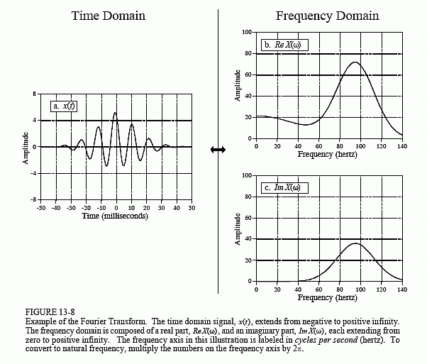
Figure 13-8 shows an example of a continuous aperiodic signal and its frequency spectrum. The time domain signal extends from negative infinity to positive infinity, while each of the frequency domain signals extends from zero to positive infinity. This frequency spectrum is shown in rectangular form (real and imaginary parts); however, the polar form (magnitude and phase) is also used with continuous signals. Just as in the discrete case, the synthesis equation describes a recipe for constructing the time domain signal using the data in the frequency domain. In mathematical form:
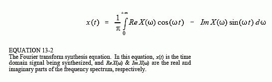
In words, the time domain signal is formed by adding (with the use of an integral) an infinite number of scaled sine and cosine waves. The real part of the frequency domain consists of the scaling factors for the cosine waves, while the imaginary part consists of the scaling factors for the sine waves. Just as with discrete signals, the synthesis equation is usually written with negative sine waves. Although the negative sign has no significance in this discussion, it is necessary to make the notation compatible with the complex mathematics described in Chapter 29. The key point to remember is that some authors put this negative sign in the equation, while others do not. Also notice that frequency is represented by the symbol, ω, a lower case
Greek omega. As you recall, this notation is called the natural frequency, and has the units of radians per second. That is, ω = 2πf, where f is the frequency in cycles per second (hertz). The natural frequency notation is favored by mathematicians and others doing signal processing by solving equations, because there are usually fewer symbols to write.
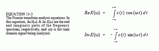
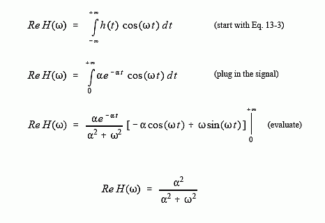
The analysis equations for continuous signals follow the same strategy as the discrete case: correlation with sine and cosine waves. The equations are:
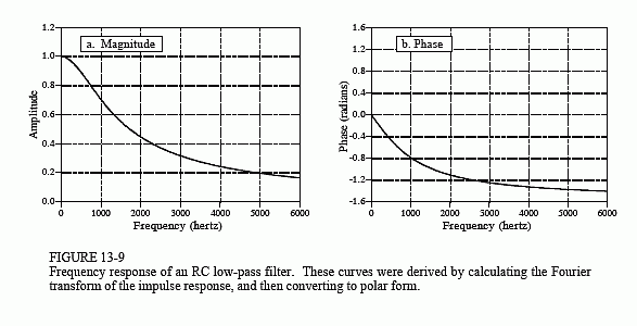
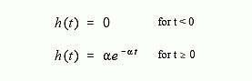
As an example of using the analysis equations, we will find the frequency response of the RC low-pass filter. This is done by taking the Fourier transform of its impulse response, previously shown in Fig. 13-4, and described by:
The frequency response is found by plugging the impulse response into the analysis equations. First, the real part:
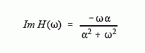
Using this same approach, the imaginary part of the frequency response is calculated to be:
Just as with discrete signals, the rectangular representation of the frequency domain is great for mathematical manipulation, but difficult for human understanding. The situation can be remedied by converting into polar notation with the standard relations: MagH(ω) = [ReH(ω2) + ImH(ω2)]1/2 and Phase H(ω) = arctan[ReH(ω)/ImH(ω)]. Working through the algebra provides the frequency response of the RC low-pass filter as magnitude and phase (i.e., polar form):
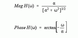
Figure 13-9 shows graphs of these curves for a cutoff frequency of 1000 hertz (i.e., α = 2π1000).