The Scientist and Engineer's Guide to
Digital Signal Processing
By Steven W. Smith, Ph.D.
Book Search

Table of contents
- 1: The Breadth and Depth of DSP
- 2: Statistics, Probability and Noise
- 3: ADC and DAC
- 4: DSP Software
- 5: Linear Systems
- 6: Convolution
- 7: Properties of Convolution
- 8: The Discrete Fourier Transform
- 9: Applications of the DFT
- 10: Fourier Transform Properties
- 11: Fourier Transform Pairs
- 12: The Fast Fourier Transform
- 13: Continuous Signal Processing
- 14: Introduction to Digital Filters
- 15: Moving Average Filters
- 16: Windowed-Sinc Filters
- 17: Custom Filters
- 18: FFT Convolution
- 19: Recursive Filters
- 20: Chebyshev Filters
- 21: Filter Comparison
- 22: Audio Processing
- 23: Image Formation & Display
- 24: Linear Image Processing
- 25: Special Imaging Techniques
- 26: Neural Networks (and more!)
- 27: Data Compression
- 28: Digital Signal Processors
- 29: Getting Started with DSPs
- 30: Complex Numbers
- 31: The Complex Fourier Transform
- 32: The Laplace Transform
- 33: The z-Transform
- 34: Explaining Benford's Law
How to order your own hardcover copy
Wouldn't you rather have a bound book instead of 640 loose pages?Your laser printer will thank you!
Order from Amazon.com.
Chapter 28: Digital Signal Processors
Digital Signal Processors are designed to quickly carry out FIR filters and similar techniques. To understand the hardware, we must first understand the algorithms. In this section we will make a detailed list of the steps needed to implement an FIR filter. In the next section we will see how DSPs are designed to perform these steps as efficiently as possible.
To start, we need to distinguish between off-line processing and real-time processing. In off-line processing, the entire input signal resides in the computer at the same time. For example, a geophysicist might use a seismometer to record the ground movement during an earthquake. After the shaking is over, the information may be read into a computer and analyzed in some way. Another example of off-line processing is medical imaging, such as computed tomography and MRI. The data set is acquired while the patient is inside the machine, but the image reconstruction may be delayed until a later time. The key point is that all of the information is simultaneously available to the processing program. This is common in scientific research and engineering, but not in consumer products. Off-line processing is the realm of personal computers and mainframes.
In real-time processing, the output signal is produced at the same time that the input signal is being acquired. For example, this is needed in telephone communication, hearing aids, and radar. These applications must have the information immediately available, although it can be delayed by a short amount. For instance, a 10 millisecond delay in a telephone call cannot be detected by the speaker or listener. Likewise, it makes no difference if a radar signal is delayed by a few seconds before being displayed to the operator. Real-time applications input a sample, perform the algorithm, and output a sample, over-and-over. Alternatively, they may input a group
of samples, perform the algorithm, and output a group of samples. This is the world of Digital Signal Processors.
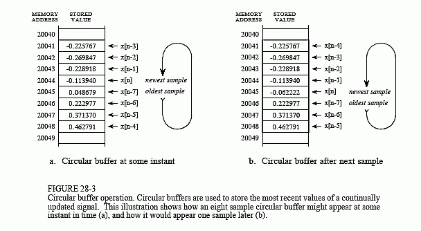
Now look back at Fig. 28-2 and imagine that this is an FIR filter being implemented in real-time. To calculate the output sample, we must have access to a certain number of the most recent samples from the input. For example, suppose we use eight coefficients in this filter, a0, a1, … a7. This means we must know the value of the eight most recent samples from the input signal, x[n], x[n-1], … x[n-7]. These eight samples must be stored in memory and continually updated as new samples are acquired. What is the best way to manage these stored samples? The answer is circular buffering.
Figure 28-3 illustrates an eight sample circular buffer. We have placed this circular buffer in eight consecutive memory locations, 20041 to 20048. Figure (a) shows how the eight samples from the input might be stored at one particular instant in time, while (b) shows the changes after the next sample is acquired. The idea of circular buffering is that the end of this linear array is connected to its beginning; memory location 20041 is viewed as being next to 20048, just as 20044 is next to 20045. You keep track of the array by a pointer (a variable whose value is an address) that indicates where the most recent sample resides. For instance, in (a) the pointer contains the address 20044, while in (b) it contains 20045. When a new sample is acquired, it replaces the oldest sample in the array, and the pointer is moved one address ahead. Circular buffers are efficient because only one value needs to be changed when a new sample is acquired.
Four parameters are needed to manage a circular buffer. First, there must be a pointer that indicates the start of the circular buffer in memory (in this example, 20041). Second, there must be a pointer indicating the end of the array (e.g., 20048), or a variable that holds its length (e.g., 8). Third, the step size of the memory addressing must be specified. In Fig. 28-3 the step size is one, for example: address 20043 contains one sample, address 20044 contains the next sample, and so on. This is frequently not the case. For instance, the addressing may refer to bytes, and each sample may require two or four bytes to hold its value. In these cases, the step size would need to be two or four, respectively.
These three values define the size and configuration of the circular buffer, and will not change during the program operation. The fourth value, the pointer to the most recent sample, must be modified as each new sample is acquired. In other words, there must be program logic that controls how this fourth value is updated based on the value of the first three values. While this logic is quite simple, it must be very fast. This is the whole point of this discussion; DSPs should be optimized at managing circular buffers to achieve the highest possible execution speed.
As an aside, circular buffering is also useful in off-line processing. Consider a program where both the input and the output signals are completely contained in memory. Circular buffering isn't needed for a convolution calculation, because every sample can be immediately accessed. However, many algorithms are implemented in stages, with an intermediate signal being created between each stage. For instance, a recursive filter carried out as a series of biquads operates in this way. The brute force method is to store the entire length of each intermediate signal in memory. Circular buffering provides another option: store only those intermediate samples needed for the calculation at hand. This reduces the required amount of memory, at the expense of a more complicated algorithm. The important idea is that circular buffers are useful for off-line processing, but critical for real-time applications.
Now we can look at the steps needed to implement an FIR filter using circular buffers for both the input signal and the coefficients. This list may seem trivial and overexamined- it's not! The efficient handling of these individual tasks is what separates a DSP from a traditional microprocessor. For each new sample, all the following steps need to be taken:
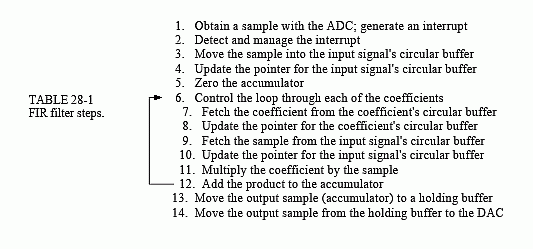
The goal is to make these steps execute quickly. Since steps 6-12 will be repeated many times (once for each coefficient in the filter), special attention must be given to these operations. Traditional microprocessors must generally carry out these 14 steps in serial (one after another), while DSPs are designed to perform them in parallel. In some cases, all of the operations within the loop (steps 6-12) can be completed in a single clock cycle. Let's look at the internal architecture that allows this magnificent performance.