The Scientist and Engineer's Guide to
Digital Signal Processing
By Steven W. Smith, Ph.D.
Book Search
Table of contents
- 1: The Breadth and Depth of DSP
- 2: Statistics, Probability and Noise
- 3: ADC and DAC
- 4: DSP Software
- 5: Linear Systems
- 6: Convolution
- 7: Properties of Convolution
- 8: The Discrete Fourier Transform
- 9: Applications of the DFT
- 10: Fourier Transform Properties
- 11: Fourier Transform Pairs
- 12: The Fast Fourier Transform
- 13: Continuous Signal Processing
- 14: Introduction to Digital Filters
- 15: Moving Average Filters
- 16: Windowed-Sinc Filters
- 17: Custom Filters
- 18: FFT Convolution
- 19: Recursive Filters
- 20: Chebyshev Filters
- 21: Filter Comparison
- 22: Audio Processing
- 23: Image Formation & Display
- 24: Linear Image Processing
- 25: Special Imaging Techniques
- 26: Neural Networks (and more!)
- 27: Data Compression
- 28: Digital Signal Processors
- 29: Getting Started with DSPs
- 30: Complex Numbers
- 31: The Complex Fourier Transform
- 32: The Laplace Transform
- 33: The z-Transform
- 34: Explaining Benford's Law
How to order your own hardcover copy
Wouldn't you rather have a bound book instead of 640 loose pages?Your laser printer will thank you!
Order from Amazon.com.
Chapter 17: Custom Filters
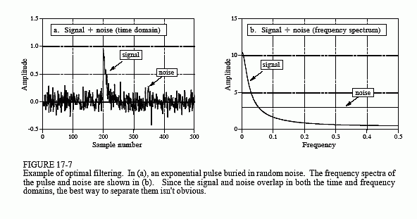
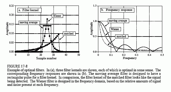
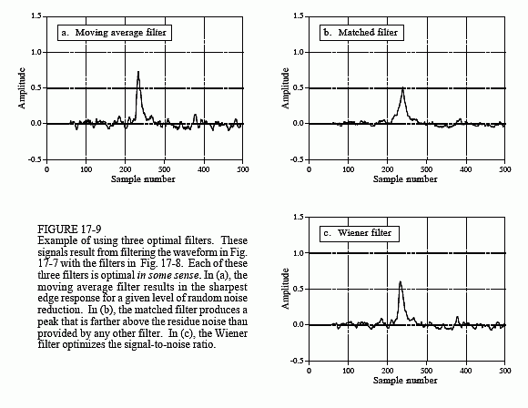
Figure 17-7a illustrates a common filtering problem: trying to extract a waveform (in this example, an exponential pulse) buried in random noise. As shown in (b), this problem is no easier in the frequency domain. The signal has a spectrum composed mainly of low frequency components. In comparison, the spectrum of the noise is white (the same amplitude at all frequencies). Since the spectra of the signal and noise overlap, it is not clear how the two can best be separated. In fact, the real question is how to define what "best" means. We will look at three filters, each of which is "best" (optimal) in a different way. Figure 17-8 shows the filter kernel and frequency response for each of these filters. Figure 17-9 shows the result of using these filters on the example waveform of Fig. 17-7a.
The moving average filter is the topic of Chapter 15. As you recall, each output point produced by the moving average filter is the average of a certain number of points from the input signal. This makes the filter kernel a rectangular pulse with an amplitude equal to the reciprocal of the number of points in the average. The moving average filter is optimal in the sense that it provides the fastest step response for a given noise reduction.
The matched filter was previously discussed in Chapter 7. As shown in Fig. 17-8a, the filter kernel of the matched filter is the same as the target signal


being detected, except it has been flipped left-for-right. The idea behind the matched filter is correlation, and this flip is required to perform correlation using convolution. The amplitude of each point in the output signal is a measure of how well the filter kernel matches the corresponding section of the input signal. Recall that the output of a matched filter does not necessarily look like the signal being detected. This doesn't really matter; if a matched filter is used, the shape of the target signal must already be known. The matched filter is optimal in the sense that the top of the peak is farther above the noise than can be achieved with any other linear filter (see Fig. 17-9b).
The Wiener filter (named after the optimal estimation theory of Norbert Wiener) separates signals based on their frequency spectra. As shown in Fig. 17-7b, at some frequencies there is mostly signal, while at others there is mostly noise. It seems logical that the "mostly signal" frequencies should be passed through the filter, while the "mostly noise" frequencies should be blocked. The Wiener filter takes this idea a step further; the gain of the filter at each frequency is determined by the relative amount of signal and noise at that frequency:

This relation is used to convert the spectra in Fig. 17-7b into the Wiener filter's frequency response in Fig. 17-8b. The Wiener filter is optimal in the sense that it maximizes the ratio of the signal power to the noise power

(over the length of the signal, not at each individual point). An appropriate filter kernel is designed from the Wiener frequency response using the custom method.
While the ideas behind these optimal filters are mathematically elegant, they often fail in practicality. This isn't to say they should never be used.
The point is, don't hear the word "optimal" and stop thinking. Let's look at several reasons why you might not want to use them.
First, the difference between the signals in Fig. 17-9 is very unimpressive. In fact, if you weren't told what parameters were being optimized, you probably couldn't tell by looking at the signals. This is usually the case for problems involving overlapping frequency spectra. The small amount of extra performance obtained from an optimal filter may not be worth the the increased program complexity, the extra design effort, or the longer execution time.
Second: The Wiener and matched filters are completely determined by the characteristics of the problem. Other filters, such as the windowed-sinc and moving average, can be tailored to your liking. Optimal filter advocates would claim that this diddling can only reduce the effectiveness of the filter. This is very arguable. Remember, each of these filters is optimal in one specific way (i.e., "in some sense"). This is seldom sufficient to claim that the entire problem has been optimized, especially if the resulting signals are interpreted by a human observer. For instance, a biomedical engineer might use a Wiener filter to maximize the signal-to-noise ratio in an electro-cardiogram. However, it is not obvious that this also optimizes a physician's ability to detect irregular heart activity by looking at the signal.
Third: The Wiener and matched filter must be carried out by convolution, making them extremely slow to execute. Even with the speed improvements discussed in the next chapter (FFT convolution), the computation time can be excessively long. In comparison, recursive filters (such as the moving average or others presented in Chapter 19) are much faster, and may provide an acceptable level of performance.
