The Scientist and Engineer's Guide to
Digital Signal Processing
By Steven W. Smith, Ph.D.
Book Search

Table of contents
- 1: The Breadth and Depth of DSP
- 2: Statistics, Probability and Noise
- 3: ADC and DAC
- 4: DSP Software
- 5: Linear Systems
- 6: Convolution
- 7: Properties of Convolution
- 8: The Discrete Fourier Transform
- 9: Applications of the DFT
- 10: Fourier Transform Properties
- 11: Fourier Transform Pairs
- 12: The Fast Fourier Transform
- 13: Continuous Signal Processing
- 14: Introduction to Digital Filters
- 15: Moving Average Filters
- 16: Windowed-Sinc Filters
- 17: Custom Filters
- 18: FFT Convolution
- 19: Recursive Filters
- 20: Chebyshev Filters
- 21: Filter Comparison
- 22: Audio Processing
- 23: Image Formation & Display
- 24: Linear Image Processing
- 25: Special Imaging Techniques
- 26: Neural Networks (and more!)
- 27: Data Compression
- 28: Digital Signal Processors
- 29: Getting Started with DSPs
- 30: Complex Numbers
- 31: The Complex Fourier Transform
- 32: The Laplace Transform
- 33: The z-Transform
- 34: Explaining Benford's Law
How to order your own hardcover copy
Wouldn't you rather have a bound book instead of 640 loose pages?Your laser printer will thank you!
Order from Amazon.com.
Chapter 23: Image Formation & Display
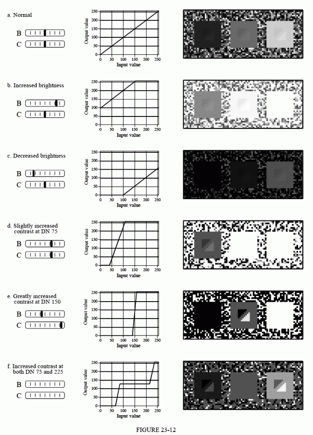
The last image, Fig. 23-12f, is different from the rest. Rather than having a slope in the curve over one range of input values, it has a slope in the curve over two ranges. This allows the display to simultaneously show the triangles in both the left and the right squares. Of course, this results in saturation of the pixel values that are not near these digital numbers. Notice that the slide bars for contrast and brightness are not shown in (f); this display is beyond what brightness and contrast adjustments can provide.
Taking this approach further results in a powerful technique for improving the appearance of images: the grayscale transform. The idea is to increase the contrast at pixel values of interest, at the expense of the pixel values we don't care about. This is done by defining the relative importance of each of the 0 to 255 possible pixel values. The more important the value, the greater its contrast is made in the displayed image. An example will show a systematic way of implementing this procedure.
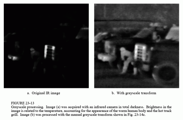
The image in Fig. 23-13a was acquired in total darkness by using a CCD camera that is sensitive in the far infrared. The parameter being imaged is temperature: the hotter the object, the more infrared energy it emits and the brighter it appears in the image. This accounts for the background being very black (cold), the body being gray (warm), and the truck grill being white (hot). These systems are great for the military and police; you can see the other guy when he can't even see himself! The image in (a) is difficult to view because of the uneven distribution of pixel values. Most of the image is so dark that details cannot be seen in the scene. On the other end, the grill is near white saturation.
The histogram of this image is displayed in Fig. 23-14a, showing that the background, human, and grill have reasonably separate values. In this example, we will increase the contrast in the background and the grill, at the expense of everything else, including the human body. Figure (b) represents this strategy. We declare that the lowest pixel values, the background, will have a relative contrast of twelve. Likewise, the highest pixel values, the grill, will have a relative contrast of six. The body will have a relative contrast of one, with a staircase transition between the regions. All these values are determined by trial and error.
The grayscale transform resulting from this strategy is shown in (c), labeled manual. It is found by taking the running sum (i.e., the discrete integral) of the curve in (b), and then normalizing so that it has a value of 255 at the
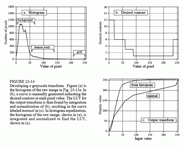
right side. Why take the integral to find the required curve? Think of it this way: The contrast at a particular pixel value is equal to the slope of the output transform. That is, we want (b) to be the derivative (slope) of (c). This means that (c) must be the integral of (b).
Passing the image in Fig. 23-13a through this manually determined grayscale transform produces the image in (b). The background has been made lighter, the grill has been made darker, and both have better contrast. These improvements are at the expense of the body's contrast, producing a less detailed image of the intruder (although it can't get much worse than in the original image).
Grayscale transforms can significantly improve the viewability of an image. The problem is, they can require a great deal of trial and error. Histogram equalization is a way to automate the procedure. Notice that the histogram in (a) and the contrast weighting curve in (b) have the same general shape. Histogram equalization blindly uses the histogram as the contrast weighing curve, eliminating the need for human judgement. That is, the output transform is found by integration and normalization of the histogram, rather than a manually generated curve. This results in the greatest contrast being given to those values that have the greatest number of pixels.
Histogram equalization is an interesting mathematical procedure because it maximizes the entropy of the image, a measure of how much information is transmitted by a fixed number of bits. The fault with histogram equalization is that it mistakes the shear number of pixels at a certain value with the importance of the pixels at that value. For example, the truck grill and human intruder are the most prominent features in Fig. 23-13. In spite of this, histogram equalization would almost completely ignore these objects because they contain relatively few pixels. Histogram equalization is quick and easy. Just remember, if it doesn't work well, a manually generated curve will probably do much better.