The Scientist and Engineer's Guide to
Digital Signal Processing
By Steven W. Smith, Ph.D.
Book Search

Table of contents
- 1: The Breadth and Depth of DSP
- 2: Statistics, Probability and Noise
- 3: ADC and DAC
- 4: DSP Software
- 5: Linear Systems
- 6: Convolution
- 7: Properties of Convolution
- 8: The Discrete Fourier Transform
- 9: Applications of the DFT
- 10: Fourier Transform Properties
- 11: Fourier Transform Pairs
- 12: The Fast Fourier Transform
- 13: Continuous Signal Processing
- 14: Introduction to Digital Filters
- 15: Moving Average Filters
- 16: Windowed-Sinc Filters
- 17: Custom Filters
- 18: FFT Convolution
- 19: Recursive Filters
- 20: Chebyshev Filters
- 21: Filter Comparison
- 22: Audio Processing
- 23: Image Formation & Display
- 24: Linear Image Processing
- 25: Special Imaging Techniques
- 26: Neural Networks (and more!)
- 27: Data Compression
- 28: Digital Signal Processors
- 29: Getting Started with DSPs
- 30: Complex Numbers
- 31: The Complex Fourier Transform
- 32: The Laplace Transform
- 33: The z-Transform
- 34: Explaining Benford's Law
How to order your own hardcover copy
Wouldn't you rather have a bound book instead of 640 loose pages?Your laser printer will thank you!
Order from Amazon.com.
Chapter 26: Neural Networks (and more!)
So, how does it work? The training program for vowel recognition was run three times using different random values for the initial weights. About one hour is required to complete the 800 iterations on a 100 MHz Pentium personnel computer. Figure 26-9 shows how the error of the network, ESUM, changes over this period. The gradual decline indicates that the network is learning the task, and that the weights reach a near optimal value after several hundred iterations. Each trial produces a different solution to the problem, with a different final performance. This is analogous to the paratrooper starting at different locations, and thereby ending up at the bottom of different valleys. Just as some valleys are deeper than others, some neural network solutions are better than others. This means that the learning algorithm should be run several times, with the best of the group taken as the final solution.
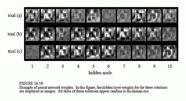
In Fig. 26-10, the hidden layer weights of the three solutions are displayed as images. This means the first action taken by the neural network is to correlate (multiply and sum) these images with the input signal. They look like random noise! These weights values can be shown to work, but why they work is something of a mystery. Here is something else to ponder. The human brain is composed of about 100 trillion neurons, each with an average of 10,000 interconnections. If we can't understand the simple neural network in this example, how can we study something that is at least 100,000,000,000,000 times more complex? This is 21st century research.
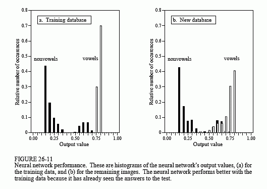
Figure 26-11a shows a histogram of the neural network's output for the 260 letters in the training set. Remember, the weights were selected to make the output near one for vowel images, and near zero otherwise. Separation has been perfectly achieved, with no overlap between the two distributions. Also notice that the vowel distribution is narrower than the nonvowel distribution. This is because we declared the target error to be five times more important than the nontarget error (see line 2220).
In comparison, Fig. 26-11b shows the histogram for images 261 through 1300 in the database. While the target and nontarget distributions are reasonably distinct, they are not completely separated. Why does the neural network perform better on the first 260 letters than the last 1040? Figure (a) is cheating! It's easy to take a test if you have already seen the answers. In other words, the neural network is recognizing specific images in the training set, not the general patterns identifying vowels from nonvowels.
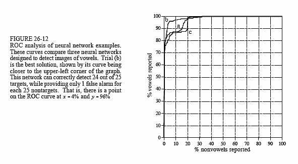
Figure 26-12 shows the performance of the three solutions, displayed as ROC curves. Trial (b) provides a significantly better network than the
other two. This is a matter of random chance depending on the initial weights used. At one threshold setting, the neural network designed in trial "b" can detect 24 out of 25 targets (i.e., 96% of the vowel images), with a false alarm rate of only 1 in 25 nontargets (i.e., 4% of the nonvowel images). Not bad considering the abstract nature of this problem, and the very general solution applied.
Some final comments on neural networks. Getting a neural network to converge during training can be tricky. If the network error (ESUM) doesn't steadily decrease, the program must be terminated, changed, and then restarted. This may take several attempts before success is reached. Three things can be changed to affect the convergence: (1) MU, (2) the magnitude of the initial random weights, and (3) the number of hidden nodes (in the order they should be changed).
The most critical item in neural network development is the validity of the training examples. For instance, when new commercial products are being developed, the only test data available are from prototypes, simulations, educated guesses, etc. If a neural network is trained on this preliminary information, it might not operate properly in the final application. Any difference between the training database and the eventual data will degrade the neural network's performance (Murphy's law for neural networks). Don't try to second guess the neural network on this issue; you can't!