The Scientist and Engineer's Guide to
Digital Signal Processing
By Steven W. Smith, Ph.D.
Book Search
Table of contents
- 1: The Breadth and Depth of DSP
- 2: Statistics, Probability and Noise
- 3: ADC and DAC
- 4: DSP Software
- 5: Linear Systems
- 6: Convolution
- 7: Properties of Convolution
- 8: The Discrete Fourier Transform
- 9: Applications of the DFT
- 10: Fourier Transform Properties
- 11: Fourier Transform Pairs
- 12: The Fast Fourier Transform
- 13: Continuous Signal Processing
- 14: Introduction to Digital Filters
- 15: Moving Average Filters
- 16: Windowed-Sinc Filters
- 17: Custom Filters
- 18: FFT Convolution
- 19: Recursive Filters
- 20: Chebyshev Filters
- 21: Filter Comparison
- 22: Audio Processing
- 23: Image Formation & Display
- 24: Linear Image Processing
- 25: Special Imaging Techniques
- 26: Neural Networks (and more!)
- 27: Data Compression
- 28: Digital Signal Processors
- 29: Getting Started with DSPs
- 30: Complex Numbers
- 31: The Complex Fourier Transform
- 32: The Laplace Transform
- 33: The z-Transform
- 34: Explaining Benford's Law
How to order your own hardcover copy
Wouldn't you rather have a bound book instead of 640 loose pages?Your laser printer will thank you!
Order from Amazon.com.
Chapter 24: Linear Image Processing
Let's use this last example to explore two-dimensional convolution in more detail. Just as with one dimensional signals, image convolution can be viewed from either the input side or the output side. As you recall from Chapter 6, the input viewpoint is the best description of how convolution works, while the output viewpoint is how most of the mathematics and algorithms are written. You need to become comfortable with both these ways of looking at the operation.
Figure 24-14 shows the input side description of image convolution. Every pixel in the input image results in a scaled and shifted PSF being added to the output image. The output image is then calculated as the sum of all the contributing PSFs. This illustration show the contribution to the output image from the point at location [r,c] in the input image. The PSF is shifted such that pixel [0,0] in the PSF aligns with pixel [r,c] in the output image. If the PSF is defined with only positive indexes, such as in this example, the shifted PSF will be entirely to the lower-right of [r,c]. Don't
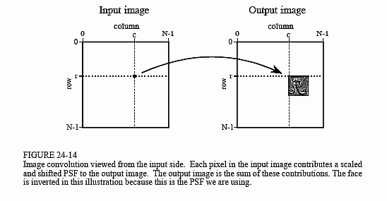
be confused by the face appearing upside down in this figure; this upside down face is the PSF we are using in this example (Fig. 24-13a). In the input side view, there is no rotation of the PSF, it is simply shifted.
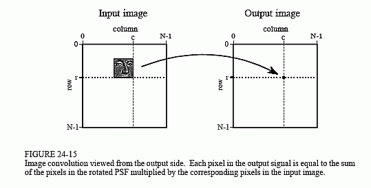
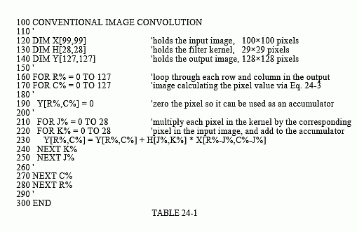
Image convolution viewed from the output is illustrated in Fig. 24-15. Each pixel in the output image, such as shown by the sample at [r,c], receives a contribution from many pixels in the input image. The PSF is rotated by 180° around pixel [0,0], and then shifted such that pixel [0,0] in the PSF is aligned with pixel [r,c] in the input image. If the PSF only uses positive indexes, it will be to the upper-left of pixel [r,c] in the input image. The value of the pixel at [r,c] in the output image is found by multiplying the pixels in the rotated PSF with the corresponding pixels in the input image, and summing the products. This procedure is given by Eq. 24-3, and in the program of Table 24-1.

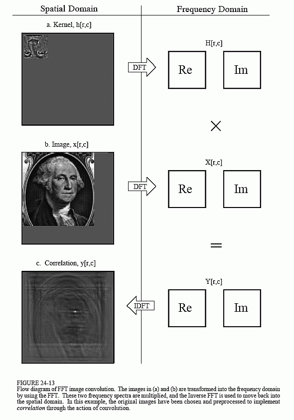
Notice that the PSF rotation resulting from the convolution has undone the rotation made in the design of the PSF. This makes the face appear upright in Fig. 24-15, allowing it to be in the same orientation as the pattern being detected in the input image. That is, we have successfully used convolution to implement correlation. Compare Fig. 24-13c with Fig. 24-15 to see how the bright spot in the correlation image signifies that the target has been detected.
FFT convolution provides the same output image as the conventional convolution program of Table 24-1. Is the reduced execution time provided by FFT convolution really worth the additional program complexity? Let's take a closer look. Figure 24-16 shows an execution time comparison between conventional convolution using floating point (labeled FP), conventional convolution using integers (labeled INT), and FFT convolution using floating point (labeled FFT). Data for two different image sizes are presented, 512×512 and 128×128.
First, notice that the execution time required for FFT convolution does not depend on the size of the kernel, resulting in flat lines in this graph. On a 100 MHz Pentium personal computer, a 128×128 image can be convolved
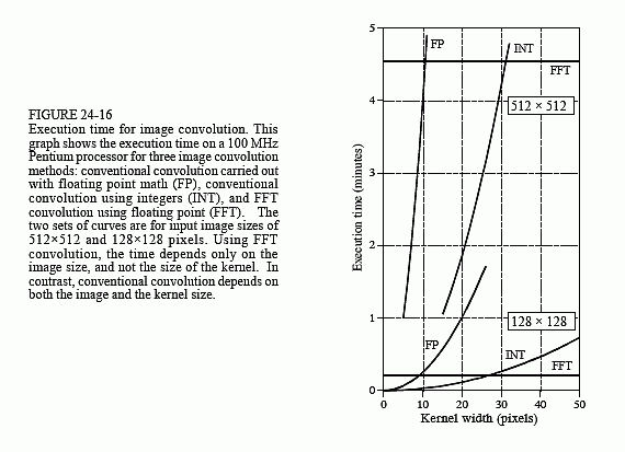
in about 15 seconds using FFT convolution, while a 512×512 image requires more than 4 minutes. Adding up the number of calculations shows that the execution time for FFT convolution is proportional to N2Log2(N), for an N×N image. That is, a 512×512 image requires about 20 times as long as a 128×128 image.
Conventional convolution has an execution time proportional to N2M2 for an N×N image convolved with an M×M kernel. This can be understood by examining the program in Table 24-1. In other words, the execution time for conventional convolution depends very strongly on the size of the kernel used. As shown in the graph, FFT convolution is faster than conventional convolution using floating point if the kernel is larger than about 10×10 pixels. In most cases, integers can be used for conventional convolution, increasing the break-even point to about 30×30 pixels. These break-even points depend slightly on the size of the image being convolved, as shown in the graph. The concept to remember is that FFT convolution is only useful for large filter kernels.
