The Scientist and Engineer's Guide to
Digital Signal Processing
By Steven W. Smith, Ph.D.
Book Search
Table of contents
- 1: The Breadth and Depth of DSP
- 2: Statistics, Probability and Noise
- 3: ADC and DAC
- 4: DSP Software
- 5: Linear Systems
- 6: Convolution
- 7: Properties of Convolution
- 8: The Discrete Fourier Transform
- 9: Applications of the DFT
- 10: Fourier Transform Properties
- 11: Fourier Transform Pairs
- 12: The Fast Fourier Transform
- 13: Continuous Signal Processing
- 14: Introduction to Digital Filters
- 15: Moving Average Filters
- 16: Windowed-Sinc Filters
- 17: Custom Filters
- 18: FFT Convolution
- 19: Recursive Filters
- 20: Chebyshev Filters
- 21: Filter Comparison
- 22: Audio Processing
- 23: Image Formation & Display
- 24: Linear Image Processing
- 25: Special Imaging Techniques
- 26: Neural Networks (and more!)
- 27: Data Compression
- 28: Digital Signal Processors
- 29: Getting Started with DSPs
- 30: Complex Numbers
- 31: The Complex Fourier Transform
- 32: The Laplace Transform
- 33: The z-Transform
- 34: Explaining Benford's Law
How to order your own hardcover copy
Wouldn't you rather have a bound book instead of 640 loose pages?Your laser printer will thank you!
Order from Amazon.com.
Chapter 17: Custom Filters
The approach used to derive the windowed-sinc filter in the last chapter can also be used to design filters with virtually any frequency response. The only difference is how the desired response is moved from the frequency domain into the time domain. In the windowed-sinc filter, the frequency response and the filter kernel are both represented by equations, and the conversion between them is made by evaluating the mathematics of the Fourier transform. In the method presented here, both signals are represented by arrays of numbers, with a computer program (the FFT) being used to find one from the other.
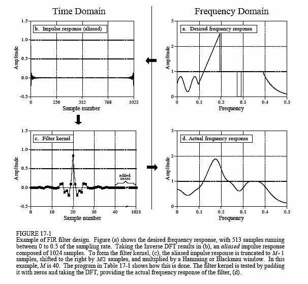
Figure 17-1 shows an example of how this works. The frequency response we want the filter to produce is shown in (a). To say the least, it is very irregular and would be virtually impossible to obtain with analog electronics. This ideal frequency response is defined by an array of numbers that have been selected, not some mathematical equation. In this example, there are 513 samples spread between 0 and 0.5 of the sampling rate. More points could be used to better represent the desired frequency response, while a smaller number may be needed to reduce the computation time during the filter design. However, these concerns are usually small, and 513 is a good length for most applications.
Besides the desired magnitude array shown in (a), there must be a corresponding phase array of the same length. In this example, the phase of the desired frequency response is entirely zero (this array is not shown in Fig. 17-1). Just as with the magnitude array, the phase array can be loaded with any arbitrary curve you would like the filter to produce. However, remember that the first and last samples (i.e., 0 and 512) of the phase array must have a value of zero (or a multiple of 2π, which is the same thing). The frequency response can also be specified in rectangular form by defining the array entries for the real and imaginary parts, instead of using the magnitude and phase.
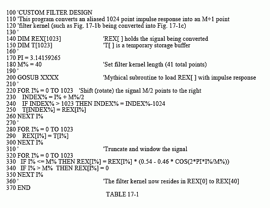
The next step is to take the Inverse DFT to move the filter into the time domain. The quickest way to do this is to convert the frequency domain to rectangular form, and then use the Inverse FFT. This results in a 1024 sample signal running from 0 to 1023, as shown in (b). This is the impulse response that corresponds to the frequency response we want; however, it is not suitable for use as a filter kernel (more about this shortly). Just as in the last chapter, it needs to be shifted, truncated, and windowed. In this example, we will design the filter kernel with M = 40, i.e., 41 points running from sample 0 to sample 40. Table 17-1 shows a computer program that converts the signal in (b) into the filter kernel shown in (c). As with the windowed-sinc filter, the points near the ends of the filter kernel are so small that they appear to be zero when plotted. Don't make the mistake of thinking they can be deleted!


The last step is to test the filter kernel. This is done by taking the DFT (using the FFT) to find the actual frequency response, as shown in (d). To obtain better resolution in the frequency domain, pad the filter kernel with zeros before the FFT. For instance, using 1024 total samples (41 in the filter kernel, plus 983 zeros), results in 513 samples between 0 and 0.5.
As shown in Fig. 17-2, the length of the filter kernel determines how well the actual frequency response matches the desired frequency response. The exceptional performance of FIR digital filters is apparent; virtually any frequency response can be obtained if a long enough filter kernel is used.
This is the entire design method; however, there is a subtle theoretical issue that needs to be clarified. Why isn't it possible to directly use the impulse response shown in 17-1b as the filter kernel? After all, if (a) is the Fourier transform of (b), wouldn't convolving an input signal with (b) produce the exact frequency response we want? The answer is no, and here's why.
When designing a custom filter, the desired frequency response is defined by the values in an array. Now consider this: what does the frequency response do between the specified points? For simplicity, two cases can be imagined, one "good" and one "bad." In the "good" case, the frequency response is a smooth curve between the defined samples. In the "bad" case, there are wild fluctuations between. As luck would have it, the impulse response in (b) corresponds to the "bad" frequency response. This can be shown by padding it with a large number of zeros, and then taking the DFT. The frequency response obtained by this method will show the erratic behavior between the originally defined samples, and look just awful.
To understand this, imagine that we force the frequency response to be what we want by defining it at an infinite number of points between 0 and 0.5. That is, we create a continuous curve. The inverse DTFT is then used to find the impulse response, which will be infinite in length. In other words, the "good" frequency response corresponds to something that cannot be represented in a computer, an infinitely long impulse response. When we represent the frequency spectrum with N/2 samples, only N points are provided in the time domain, making it unable to correctly contain the signal. The result is that the infinitely long impulse response wraps up (aliases) into the N points. When this aliasing occurs, the frequency response changes from "good" to "bad." Fortunately, windowing the N point impulse response greatly reduces this aliasing, providing a smooth curve between the frequency domain samples.
Designing a digital filter to produce a given frequency response is quite simple. The hard part is finding what frequency response to use. Let's look at some strategies used in DSP to design custom filters.
